Variance = E[I 2 ] 2pE[I] + p 2 = E[I] 2p p + p 2 = 2 2 = p-2p+ - - PowerPoint PPT Presentation

variance.1 Albert R Meyer, May 10, 2013

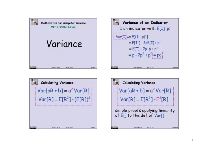
Variance

Mathematics for Computer Science

MIT 6.042J/18.062J

variance.2 Albert R Meyer, May 10, 2013

Var[I] ::= E[(I − p)2]

Variance of an Indicator

I an indicator with E[I]=p:

= E[I2] − 2pE[I] + p2

= E[I] − 2p ⋅ p + p2

2 2

p-2p + p pq = =

variance.3 Albert R Meyer, May 10, 2013

Calculating Variance

Var[aR + b] = a2 Var[R] Var[R] = E[R2] -(E[R])2

variance.4 Albert R Meyer, May 10, 2013

Calculating Variance

simple proofs applying linearity

• f E[] to the def of Var[]

Var[aR + b] = a2 Var[R] Var[R] = E[R2] -E2[R]

1

=

variance.5 Albert R Meyer, May 10, 2013

proof of 2nd Variance Formula

Var[R] ::= E[(R - μ)2]

= E[R 2 - 2μ R + μ2] = E[R2] − 2μ·E[R] + E[μ2] = E[R2] − 2μ·μ + μ2 = E[R2] − μ2

= E[R2] − E2[R]

variance.6 Albert R Meyer, May 10, 2013

Space Station Mir

Destructs with probability p in any given hour

E[F] = 1/p (Mean Time to Fail) Var[F] = ?

Variance of Time to Failure Variance of Time to Failure

E[F2] ::= ∑

∞

k2 ⋅Pr[F2 =k2] Pr[F = k] = qk−1p

k=1

Var[F] = E[F

2] − E2[F]

∞

= ∑k2 ⋅Pr[F =k] F = 1, 2, 3,…, k ,...

k=1 ∞

p

F2 = 1, 4, 9,…, k2,…

= ∑k2qk q k

=

k=0

has closed form

Albert R Meyer, May 10, 2013 variance.7 Albert R Meyer, May 10, 2013 variance.8

2

variance.9 Albert R Meyer, May 10, 2013

E[F2 |F =1]⋅Pr[F =1] +E[F2 |F > 1]⋅Pr[F > 1]

Variance of Time to Failure

total expectation approach: E[F2] =

variance.10 Albert R Meyer, May 10, 2013

lemma: For F = time to failure, ,

E[ g(F) |F > n]

g : R → R

Conditional time to failure

variance.11 Albert R Meyer, May 10, 2013

E[F2 |F > 1] =E[(F + 1)2]

lemma: For F = time to failure, ,

E[ g(F) |F > n] = E[ g(F + n)]

g : R → R

Conditional time to failure

Corollary:

variance.12 Albert R Meyer, May 10, 2013

E[F2 |F =1]⋅Pr[F =1] +E[F2 |F > 1]⋅Pr[F > 1]

Variance of Time to Failure

total expectation approach: E[F2] =

3

variance.13 Albert R Meyer, May 10, 2013

1 ⋅ p +E[F2 |F > 1]⋅Pr[F > 1]

Variance of Time to Failure

E[F2] = total expectation approach:

variance.14 Albert R Meyer, May 10, 2013

1 ⋅ p +E[(F +1)2] ⋅ q

Variance of Time to Failure

E[F2] = total expectation approach:

variance.15 Albert R Meyer, May 10, 2013

1 ⋅ p + (E[F2] + 2/ p + 1) ⋅ q

Variance of Time to Failure

E[F2] = total expectation approach:

now solve for E[F2]

variance.18 Albert R Meyer, May 10, 2013

Mir1:

p = 10-4, E[F] = 104, σ < 104

so by Chebyshev Pr[lasts ≥ 4 104 hours] ≤ 1/4 Mean Time to Failure

Var[F] = 1 p 1 p -1      

4

Mean Time to Failure

1  1  Var[F] =

• 1

p   p  

Mir1:

p = 10-4, E[F] = 104, σ < 104

so by Chebyshev Pr[lasts ≥ 4.6 years ] ≤ 1/4

Albert R Meyer, May 10, 2013 variance.19

Calculating Variance

Pairwise Independent Additivity

providing R1,R2,…,Rn are pairwise independent Var[R1 + R2 ++ R

n]

= Var[R1] + Var[R2] ++ Var[Rn]

variance.20 Albert R Meyer, May 10, 2013

again, a simple proof applying linearity of E[] to the def of Var[]

5

MIT OpenCourseWare http://ocw.mit.edu

6.042J / 18.062J Mathematics for Computer Science

Spring 2015 For information about citing these materials or our Terms of Use, visit: http://ocw.mit.edu/terms.