Announcements: Discussion via Zoom; see Canvas for link Project 4 - - PowerPoint PPT Presentation

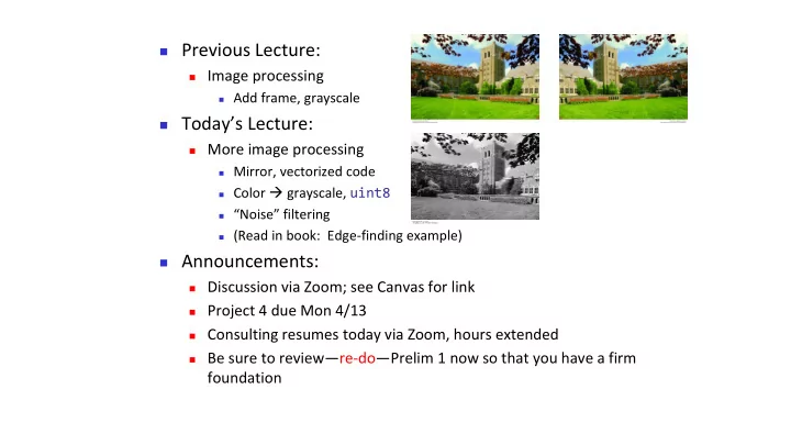
◼ Previous Lecture:

◼ Image processing

◼ Add frame, grayscale

◼ Today’s Lecture:

◼ More image processing

◼ Mirror, vectorized code ◼ Color → grayscale, uint8 ◼ “Noise” filtering ◼ (Read in book: Edge-finding example)

◼ Announcements:

◼ Discussion via Zoom; see Canvas for link ◼ Project 4 due Mon 4/13 ◼ Consulting resumes today via Zoom, hours extended ◼ Be sure to review—re-do—Prelim 1 now so that you have a firm

foundation

Where did we leave off? How to put a picture in a frame Two approaches:

1.

Ask every pixel whether it is covered by the frame

◼

Easy to understand

2.

Identify which subarrays are covered by the frame

◼

More efficient; easy to vectorize

Pictures as matrices

24 29 30 28 26 124 72 34 27 26 236 212 142 65 32 231 232 232 198 130 231 228 224 225 215 Pixel: an element in a matrix (location corresponds to row, column index) “Greyness”: a value in 0..255

A color picture is made up of RGB matrices → 3D array

114 114 112 112 114 111 114 115 112 113 114 113 111 109 113 111 113 115 112 113 115 114 112 111 111 112 112 111 112 112 116 117 116 114 112 115 113 112 115 114 113 112 112 112 112 110 111 113 116 115 115 115 115 115 113 111 111 113 116 114 112 113 116 117 113 112 112 113 114 113 115 116 118 118 113 112 112 113 114 114 116 116 117 117 114 114 112 112 114 115 153 153 150 150 154 151 152 153 150 151 153 152 149 147 153 151 151 153 150 151 154 153 151 150 151 152 150 149 150 150 155 156 155 152 152 155 151 150 153 153 151 150 150 150 150 148 149 151 152 151 153 153 153 153 151 149 149 151 152 150 150 151 152 153 151 150 150 151 152 151 153 154 154 154 151 150 150 151 152 152 154 154 153 153 149 149 150 150 152 153 212 212 212 212 216 213 215 216 213 213 212 211 211 209 215 213 214 216 213 213 213 212 210 209 212 214 213 212 213 212 214 215 214 214 213 216 214 213 215 212 213 212 212 212 212 210 211 213 214 211 215 215 216 216 213 211 211 213 212 210 212 213 214 215 213 212 212 213 214 213 215 216 216 216 213 212 212 213 214 214 216 216 215 215 213 213 213 213 214 215

0 ≤ A(i,j,1) ≤ 255 0 ≤ A(i,j,3) ≤ 255 0 ≤ A(i,j,2) ≤ 255 E.g., color image data is stored in a 3-d array A:

Color image 3-d Array 0 ≤ A(i,j,1) ≤ 255 0 ≤ A(i,j,3) ≤ 255 0 ≤ A(i,j,2) ≤ 255

Visualize a 3D array as a stack of “layers” which are 2D arrays Beware the two different “3”s:

◼ dims = size(A) % [720, 1280, 3] ◼ length(dims) == 3 % A has 3 dimensions: rows, columns, layers ◼ dims(3) == 3

% A has 3 layers: red, green, blue

Example: Mirror Image

LawSchool.jpg LawSchoolMirror.jpg

1.

Read LawSchool.jpg from memory and convert it into an array.

2.

Manipulate the Array.

3.

Convert the array to a jpg file and write it to memory.

Reading and writing jpg files % Read jpg image, uncompress to a % a 3D array A of type uint8 A = imread('LawSchool.jpg'); % Write 3D array B to memory as % a jpg image imwrite(B,'LawSchoolMirror.jpg')

%Store mirror image of A in array B [nr,nc,np]= size(A); for r = 1:nr for c = 1:nc B(r,c )= A(r,nc-c+1 ); end end

A B

1 5 2 4 3 3 4 2 5 1

%Store mirror image of A in array B [nr,nc,np]= size(A); for r = 1:nr for c = 1:nc for p = 1:np B(r,c,p)= A(r,nc-c+1,p); end end end

[nr,nc,np]= size(A); for r= 1:nr for c= 1:nc for p= 1:np B(r,c,p)= A(r,nc-c+1,p); end end end [nr,nc,np]= size(A); for p= 1:np for r= 1:nr for c= 1:nc B(r,c,p)= A(r,nc-c+1,p); end end end Both fragments create a mirror image of A . true false

A B

% Make mirror image of A -- the whole thing A= imread('LawSchool.jpg'); [nr,nc,np]= size(A); for r= 1:nr for c= 1:nc for p= 1:np B(r,c,p)= A(r,nc-c+1,p); end end end imshow(B) % Show 3-d array data as an image imwrite(B,'LawSchoolMirror.jpg')

% Make mirror image of A –- the whole thing A= imread('LawSchool.jpg'); [nr,nc,np]= size(A); B= zeros(nr,nc,np); % zeros returns type double B= uint8(B); % Convert B to type uint8 for r= 1:nr for c= 1:nc for p= 1:np B(r,c,p)= A(r,nc-c+1,p); end end end imshow(B) % Show 3-d array data as an image imwrite(B,'LawSchoolMirror.jpg')

Vectorized code simplifies things… Work with a whole column at a time

A B 1 6 2 5 3 4 6 5 4 1 2 3 Column c in B is column nc-c+1 in A

Consider a single matrix (just one layer) [nr,nc,np] = size(A); for c= 1:nc B(: ,c ) = A(: ,nc-c+1 ); end

all rows all rows

Consider a single matrix (just one layer) [nr,nc,np] = size(A); for c= 1:nc B(1:nr,c ) = A(1:nr,nc-c+1 ); end

Consider a single matrix (just one layer) [nr,nc,np] = size(A); for c= 1:nc B( : ,c ) = A( : ,nc-c+1 ); end

Now repeat for all layers [nr,nc,np] = size(A); for c= 1:nc B(:,c,1) = A(:,nc-c+1,1) B(:,c,2) = A(:,nc-c+1,2) B(:,c,3) = A(:,nc-c+1,3) end

Vectorized code to create a mirror image A = imread('LawSchool.jpg') [nr,nc,np] = size(A); for c= 1:nc B(:,c,1) = A(:,nc-c+1,1) B(:,c,2) = A(:,nc-c+1,2) B(:,c,3) = A(:,nc-c+1,3) end imwrite(B,'LawSchoolMirror.jpg')

Even more compact vectorized code to create a mirror image…

for c= 1:nc B(:,c,1) = A(:,nc-c+1,1) B(:,c,2) = A(:,nc-c+1,2) B(:,c,3) = A(:,nc-c+1,3) end B = A(:,nc:-1:1,:)

Example: color → black and white Can “average” the three color values to get one gray value.

Converting from color (RGB) to grayscale

R G B

Averaging the RGB values to get a gray value

.21R+.72G+.07B

R G B

Averaging the RGB values to get a gray value

A 3-d array 2-d array for i= 1:m for j= 1:n M(i,j)= .21*R(i,j ) + .72*G(i,j ) + .07*B(i,j ) end end

Averaging the RGB values to get a gray value

A 3-d array 2-d array for i= 1:m for j= 1:n M(i,j)= .21*A(i,j,1) + .72*A(i,j,2) + .07*A(i,j,3) end end

Averaging the RGB values to get a gray value

A 3-d array 2-d array for i= 1:m for j= 1:n M(i,j)= .21*A(i,j,1) + .72*A(i,j,2) + .07*A(i,j,3) end end M = .21*A(:,:,1) + .72*A(:,:,2) + .07*A(:,:,3)

Computing in type uint8

◼ Respect the range [0..255] ◼ Arithmetic on uint8’s results in uint8’s ◼ Saturation (also called “capped”)

◼ uint8(90) + uint8(200) → 255 (type uint8) ◼ uint8(90) - uint8(200) → ___ (type uint8)

◼ Rounding (not truncation)

◼ uint8(32)/uint8(3) → _____

(type uint8)

◼ Arithmetic between a uint8 and a double results in

a uint8

◼ uint8(90) + 200 → _____

(type uint8) 11 255

Here are 2 ways to calculate the average. Are gray value matrices g and h the same given uint8 image data A?

for r= 1:nr for c= 1:nc g(r,c)= A(r,c,1)/3 + A(r,c,2)/3 + ... A(r,c,3)/3; h(r,c)= ... ( A(r,c,1)+A(r,c,2)+A(r,c,3) )/3; end end

A: yes B: not quite (rounding) C: no (saturation)

Application: median filtering

How can we remove noise?

Dirty pixels look out-of-place

150 149 152 153 152 155 151 150 153 154 153 156 153 2 3 156 155 158 154 2 1 157 156 159 156 154 158 159 158 161 157 156 159 160 159 162

How to fix “bad” pixels?

• Visit each pixel
• Replace with typical values from

its neighborhood

• How to choose “typical” value?
• How big is the neighborhood?
• “Typical”: mean vs. median
• Median better for rejecting noise,

preserving edges

• Neighborhood: moving window
• f radius r

Using a radius-1 neighborhood

6 7 6 7 7 7 6 6 Before 6 7 6 7 6 7 7 6 6 After

6 6 6 6 7 7 7 7 median

Top-down design

◼ Visit each pixel ◼ Choose a new gray value equal to the median of the old gray

values in the “neighborhood”

[nr,nc] = size(A); % A is 2d array of image data B = uint8(zeros(nr,nc)); for i = 1:nr for j = 1:nc C = neighborhood of pixel (i,j) B(i,j) = median of elements in C end end

i = 1 j = 1 Original: Filtered:

Replace with the median of the values under the window.

i = 1 j = 2 Original: Filtered:

Replace with the median of the values under the window.

i = 1 j = 3 Original: Filtered:

Replace with the median of the values under the window.

i = 1 j = nc Original: Filtered:

Replace with the median of the values under the window.

i = 2 j = 1 Original: Filtered:

Replace with the median of the values under the window.

i = 2 j = 2 Original: Filtered:

Replace with the median of the values under the window.

i = nr j = nc Original: Filtered:

Replace with the median of the values under the window.

Details at a pixel (i,j) with a radius 1 “neighborhood”

6 7 6 7 7 7 6 6

Before

6 6 6 6 7 7 7 7 median i j 6 7 6 7 6 7 7 6 6

After Replace pixel (i,j) with median value

% Get median value in a matrix xMat xVec= xMat(:) % Convert matrix to vector medianVal= median(xVec) % Use built-in function

Deal with boundary issues – moving window

% Get C, the radius r % neighborhood of pixel (i,j) iMin= i-r iMax= i+r jMin= j-r jMax= j+r C= A(iMin:iMax,jMin:jMax)

nr

1

⁞

1 …

nr×nc matrix A nc

Deal with boundary issues – moving window

% Get C, the radius r % neighborhood of pixel (i,j) iMin= max( 1,i-r) iMax= min(nr,i+r) jMin= max( 1,j-r) jMax= min(nc,j+r) C= A(iMin:iMax,jMin:jMax)

1

nc

…

nr×nc matrix A nr

1

⁞

B = medianFilter(A,3)

A

Mean Filter with radius 3

Mean Filter with radius 10

Mean filter fails because the mean does not capture representative values.

150 149 152 153 152 155 151 150 153 154 153 156 153 2 3 156 155 158 154 2 1 157 156 159 156 154 158 159 158 161 157 156 159 160 159 162

85 86 87 88

mean-filtered values with radius 1 neighborhood

150 150 153 154

median-filtered values with radius 1 neighborhood

Finding Edges: read example in Sec 12.4

Identify “sharp changes” in image data—a kind of outliers. Subtracting uint8 values correctly to prevent “underflow” “Thresholding”—use a parameter to control the amount of details extracted from image

