
SLIDE 1
1
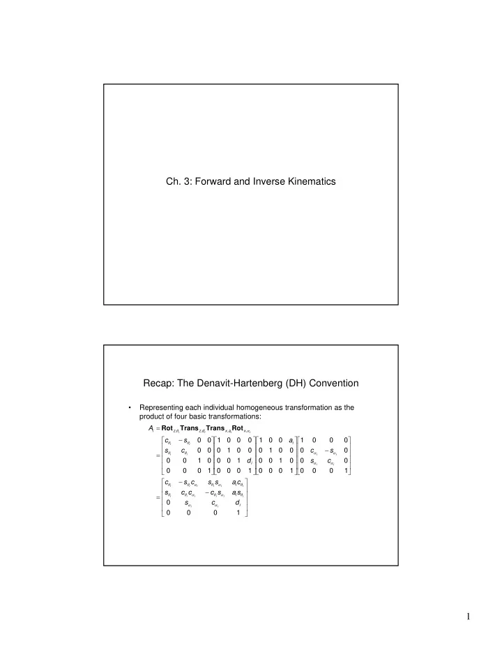
- Ch. 3: Forward and Inverse Kinematics
Recap: The Denavit-Hartenberg (DH) Convention
- Representing each individual homogeneous transformation as the
product of four basic transformations: product of four basic transformations:
⎥ ⎥ ⎤ ⎢ ⎢ ⎡ − ⎥ ⎥ ⎥ ⎥ ⎦ ⎤ ⎢ ⎢ ⎢ ⎢ ⎣ ⎡ − ⎥ ⎥ ⎥ ⎥ ⎦ ⎤ ⎢ ⎢ ⎢ ⎢ ⎣ ⎡ ⎥ ⎥ ⎥ ⎥ ⎦ ⎤ ⎢ ⎢ ⎢ ⎢ ⎣ ⎡ ⎥ ⎥ ⎥ ⎥ ⎦ ⎤ ⎢ ⎢ ⎢ ⎢ ⎣ ⎡ − = = 1 1 1 1 1 1 1 1 1 1 1 1
, , , , i i i x a x d z z i
s a s c c c s c a s s c s c c s s c a d c s s c A
i i i i i i i i i i i i i i i i i i
θ α θ α θ θ α α α α θ θ θ θ α θ
Rot Trans Trans Rot ⎥ ⎥ ⎥ ⎦ ⎢ ⎢ ⎢ ⎣ − = 1
i i
d c s s a s c c c s
i i i i i i i i
α α θ α θ α θ θ