Brownian Motion Variations and Brownian Motion with drift Today: - PowerPoint PPT Presentation

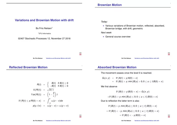
Brownian Motion Variations and Brownian Motion with drift Today: ◮ Various variations of Brownian motion, reflected, absorbed, Bo Friis Nielsen 1 Brownian bridge, with drift, geometric Next week 1 DTU Informatics ◮ General course overview 02407 Stochastic Processes 12, November 27 2018 Bo Friis Nielsen Variations and Brownian Motion with drift Bo Friis Nielsen Variations and Brownian Motion with drift Reflected Brownian Motion Absorbed Brownian Motion The movement ceases once the level 0 is reached. G t ( x , y ) = P { A ( t ) > y | A ( 0 ) = x } = P { B ( t ) > y , min { B ( u ) > 0 ; 0 ≤ u ≤ t | B ( 0 ) = x } � B ( t ) if B ( t ) ≥ 0 R ( t ) = − B ( t ) if B ( t ) < 0 We first observe � E ( R ( t )) = 2 t /π P { B ( t ) > y | B ( 0 ) = x } = G t ( x , y ) � 1 − 2 � V ar ( R ( t )) = t π + P { B ( t ) > y , min { B ( u ) ≤ 0 ; 0 ≤ u ≤ t }| B ( 0 ) = x } � y P { R ( t ) ≤ y | R ( 0 ) = x } = φ t ( z − x ) d x Due to reflection the latter term is also − y p ( y , t | x ) = φ t ( y − x ) + φ t ( y + x ) P { B ( t ) > y , min { B ( u ) ≤ 0 ; 0 ≤ u ≤ t }| B ( 0 ) = x } = P { B ( t ) < − y , min { B ( u ) ≤ 0 ; 0 ≤ u ≤ t }| B ( 0 ) = x } = P { B ( t ) < − y | B ( 0 ) = x } Bo Friis Nielsen Variations and Brownian Motion with drift Bo Friis Nielsen Variations and Brownian Motion with drift

Absorbed Brownian Motion Brownian Bridge Distribution of B ( t ); 0 ≤ t ≤ 1 conditioned on { B ( 0 ) = 0 , B ( 1 ) = 0 } . X = B ( t ) and B ( 1 ) − B ( t ) are indepedent normal variables. Summarizing we get Y = B ( 1 ) − B ( t ) + B ( t ) and X are bivariate normal. V ar ( x ) = t P { A ( t ) > y | A ( 0 ) = x } = G t ( x , y ) √ √ C ov ( X , Y ) = E ( B ( t ) B ( t ) + B ( t )( 1 − B ( t ))) = t = ρ t 1 = 1 − Φ t ( y − x ) − Φ t ( − y − x ) E ( X ) + ρσ X E ( X | Y = y = 0 ) = · ( y − E ( Y )) = 0 = Φ t ( y + x ) − Φ t ( y − x ) σ Y t ( 1 − ρ 2 ) = t ( 1 − t ) V ar ( X | Y ) = We have already seen that P { A ( t ) = 0 | A ( 0 ) = x } = 2 [ 1 − Φ t ( x )] E { B ( t ) | B ( 0 ) = 0 , B ( 1 ) = 0 } = 0 V ar { B ( t ) | B ( 0 ) = 0 , B ( 1 ) = 0 } = t ( 1 − t ) C ov { B ( s ) , B ( t ) | B ( 0 ) = 0 , B ( 1 ) = 0 } = s ( 1 − t ) The process is Gaussian Bo Friis Nielsen Variations and Brownian Motion with drift Bo Friis Nielsen Variations and Brownian Motion with drift Brownian Motion with Drift Absorption Probabilities T ab = min { t ≥ 0 ; X ( t ) = a or X ( t ) = b } u ( x ) = P { X ( T ab ) = b | X ( 0 ) = x } We assume that absorption has not occurred at (∆ t , x + ∆ X ) X ( t ) = µ t + σ B ( t ) u ( x ) = E ( u ( x + ∆ X )) ◮ A continuous sample path process with independent Taylor series expansion of right hand side increments � u ( x ) + u ′ ( x )∆( X ) + 1 (∆ X ) 2 �� 2 u ”( x )(∆ X ) 2 + o � µ t , σ 2 t ◮ X ( t + s ) − X ( s ) ∼ N � � u ( x ) = E � y − µ t − x � u ( x ) + u ′ ( x ) E [∆( X )] + 1 P { X ( t ) ≤ y | X ( 0 ) = x } = Φ √ � (∆ X ) 2 � � � (∆ X ) 2 �� = 2 u ”( x ) E + E o σ t � (∆ X ) 2 � = σ 2 ∆ t + ( µ ∆ t ) 2 E [∆( X )] = µ ∆ t , E µ u ′ ( x ) + 1 u ( x ) = Ae − 2 µ x σ 2 + B 2 σ 2 u ”( x ) = 0 , Bo Friis Nielsen Variations and Brownian Motion with drift Bo Friis Nielsen Variations and Brownian Motion with drift

Absorption probabilities Theorem 8.1 Mean Time to Absorption T ab = min { t ≥ 0 ; X ( t ) = a or X ( t ) = b } µ u ′ ( x ) + 1 u ( x ) = Ae − 2 µ x 2 σ 2 u ”( x ) = 0 , σ 2 + B v ( x ) = E { T ab | X ( 0 ) = x } v ( x ) = ∆ t + E ( v ( x + ∆ X )) u ( x ) = Ae − 2 µ x σ 2 + B , u ( a ) = 0 , u ( b ) = 1 1 + µ v ′ ( x ) + 1 2 σ 2 v ”( x ) = 0 u ( x ) = e − 2 µ x σ 2 − e − 2 µ a σ 2 e − 2 µ b σ 2 − e − 2 µ a v ( a ) = v ( b ) = 0 σ 2 v ( x ) = 1 µ [ u ( x )( b − a ) − ( x − a )] Bo Friis Nielsen Variations and Brownian Motion with drift Bo Friis Nielsen Variations and Brownian Motion with drift Maximum of Brownian Motion with Negative Drift Geometric Brownian Motion We assume µ < 0, using Theorem 8.2.1 Z ( t ) = ze ( α − 1 2 σ 2 ) t + σ B ( t ) ( Z ( 0 ) = z ) u ( x ) = e − 2 µ x σ 2 − e − 2 µ a � α − 1 � σ 2 2 σ 2 , σ 2 X ( t ) = log ( z ) + log ( Z ( t ) , X ( t ) ∼ N e − 2 µ b σ 2 − e − 2 µ a σ 2 E ( Z ( t )) = ze ( α − 1 � e σ B ( t ) � = ze ( α − 1 2 σ 2 ) t e ( 1 2 σ 2 ) t = ze α t 2 σ 2 ) t E we get 2 σ 2 we have that Z ( t ) → 0 with probability 1 For α < 1 e − 2 µ · 0 σ 2 − e − 2 µ a σ 2 = e − 2 | µ | σ 2 y P { max 0 ≤ t X ( t ) > y } = lim e − 2 µ y σ 2 − e − 2 µ a a →−∞ V ar ( Z ( t )) = z 2 e 2 α t � e σ 2 t − 1 � σ 2 Bo Friis Nielsen Variations and Brownian Motion with drift Bo Friis Nielsen Variations and Brownian Motion with drift