
SLIDE 1
4
IIT-Bombay Lecture 22 M. Shojaei Baghini
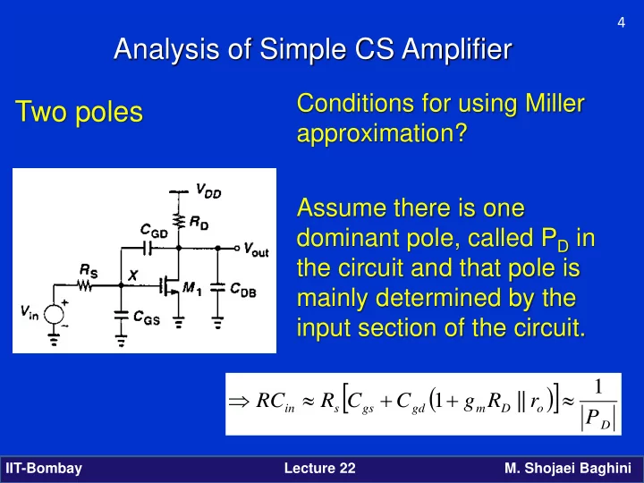
Conditions for using Miller approximation? Assume there is one dominant pole, called PD in the circuit and that pole is mainly determined by the input section of the circuit. ( )
[ ]
D
- D
m gd gs s in