An Empirical Study of Delay Introduction Jitter Management Policies - - PDF document

1

An Empirical Study of Delay Jitter Management Policies

• D. Stone and K. Jeffay

Computer Science Department University of North Carolina, Chapel Hill ACM Multimedia Systems Volume 2, Number 6 January 1995

Introduction

• Want to support interactive audio
• “Last mile” is LAN (including bridges, hubs) to

desktop – Study that – (Me: 1995 LANs looked a lot like today’s WANs)

• Transition times vary, causing gaps in playout

– Can ameliorate with display queue (buffer)

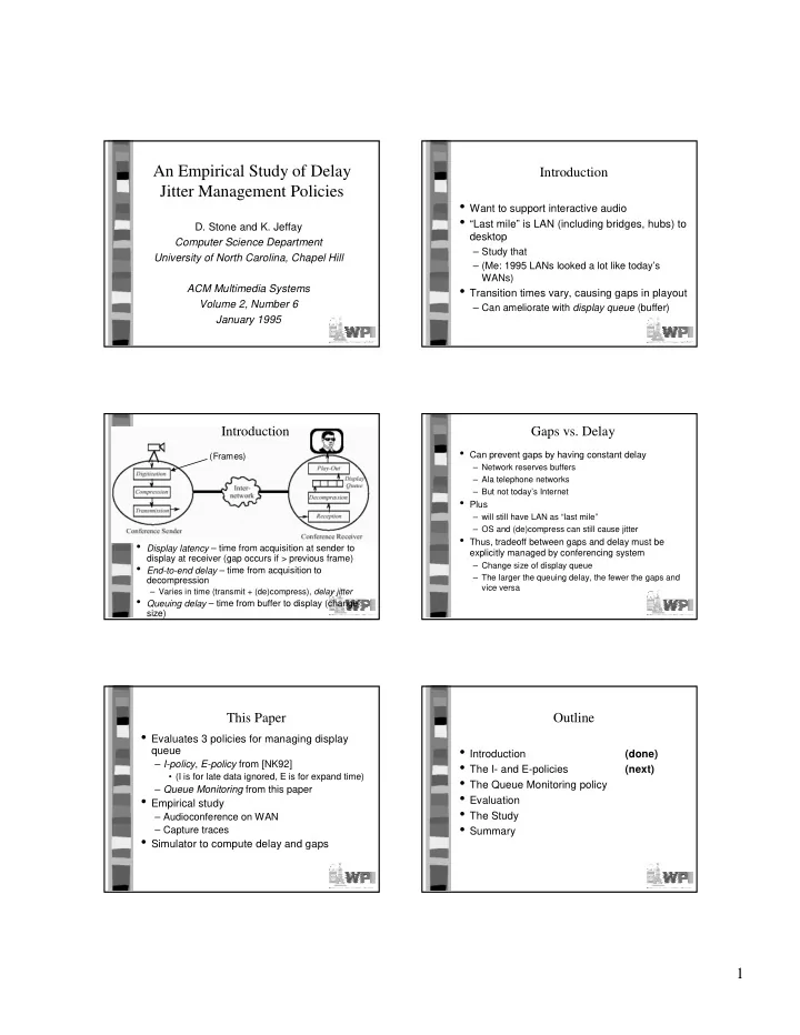
(Frames)

• Display latency – time from acquisition at sender to

display at receiver (gap occurs if > previous frame)

• End-to-end delay – time from acquisition to

decompression

– Varies in time (transmit + (de)compress), delay jitter

• Queuing delay – time from buffer to display (change

size)

Introduction Gaps vs. Delay

• Can prevent gaps by having constant delay

– Network reserves buffers – Ala telephone networks – But not today’s Internet

• Plus

– will still have LAN as “last mile” – OS and (de)compress can still cause jitter

• Thus, tradeoff between gaps and delay must be

explicitly managed by conferencing system

– Change size of display queue – The larger the queuing delay, the fewer the gaps and vice versa

This Paper

• Evaluates 3 policies for managing display

queue – I-policy, E-policy from [NK92]

• (I is for late data ignored, E is for expand time)

– Queue Monitoring from this paper

• Empirical study

– Audioconference on WAN – Capture traces

• Simulator to compute delay and gaps

Outline

• Introduction

(done)

• The I- and E-policies

(next)

• The Queue Monitoring policy
• Evaluation
• The Study
• Summary

2

The Effect of Delay Jitter

• If display latency worse than largest end-to-

end latency, then no gaps – (When is this not what we want?)

• Playout with low latency and some gaps

preferable to high-latency and no gaps

• What if a frame arrives after its playout time?
• Two choices:

– I-Policy – single fixed latency, so discard – E-Policy – late frames always displayed, so expand playout time

I-Policy

(Queue parameter is 2)

(3 gaps, display latency of 2)

E-Policy

(1 gaps, display latency of 3 at end)

I-Policy (2)

One event, but latency still low

(e, f, g, … )

E-Policy (2)

One event, latency higher

Policy Summary

• Display latency chosen implicitly with E-policy
• Choose it explicitly with I-policy
• What is the right display latency amount?

– Depends on application

• Example: surgeon viewing operation vs.

televised lecture

– Depends on network and machines

• Can vary across long run
• So, need a policy that allows display latency

to be chosen dynamically

3

Outline

• Introduction

(done)

• The I- and E-policies

(done)

• The Queue Monitoring policy

(next)

• Evaluation
• The Study
• Summary

Adjusting Display Latency

• Audioconference with silence detection can

be modeled as series of talkspurts – Sound and then silence

• Adjust display latency between talkspurts
• NK92 said observe last m fragments, discard

k largest delays and choose display latency as greatest delay – Recommend m>40 and k=0.07*m

• Other approaches as in [MKT98]

Monitor the Queue

• Measuring the end-to-end latency is difficult because

needs synchronized clocks

• Instead, observe length of display queue over time

– If end-to-end delays constant, queue size will remain the same – If end-to-end delay increases, queue shrinks – If end-to-end delay decreases, queue expands

• If queue length > 2 for some time, can reduce queue

without causing a gap

– “some time” is parameter, n, in frame times – Implement with counters for each of m frames in queue – If any > n, discard a frame and reset

• (keep queue at least 2)

– Use QM-120 as default

Outline

• Introduction

(done)

• The I- and E-policies

(done)

• The Queue Monitoring policy

(done)

• Evaluation

(next)

• The Study
• Summary

Comparing Policies

• If A has lower latency and gaps than B, then

better

• If A lower latency, but higher gaps than which

is better? – Depends upon relative amounts – Resolution – Application requirements – Few standards

Comparing Policies

• Assume:

– Differences in latency of 15ms or more significant – Difference in gap rate of 1 per minute significant

• A is better than B if either gap or latency better and

the other is the same

• Equal if same in both dimensions
• Incomparable if each is better in one dimension
• Note, for I-policy, synchronized clocks difficult.

– Instead, delay first packet for amount of time (try 2 and 3 frames in this paper)

4

Outline

• Introduction

(done)

• The I- and E-policies

(done)

• The Queue Monitoring policy

(done)

• Evaluation

(done)

• The Study

(next)

• Summary

The Study

• Run videoconference

– Use audio only

• Record end-to-end delay
• Input into simulator to evaluate policy

Videoconference

• Built at UNC
• Runs on IBM PS/2
• Uses UDP
• IBM-Intel ActionMedia 750

– 30 fps, 256x240, 8-bit color (6-8k frames) – Audio 60 fps, 128 kb/second into 16.5ms frames (266 byte packets)

Network

• 10 Mb Ethernets and 16 Mb token rings
• 400 Unix workstations and Macs
• NFS and AFS
• Send machine ! token-ring ! gateway !

department ethernet ! bridge ! department ethernet ! gateway ! token-ring ! display machine

Data

• Gather data for 10 minute interval
• 24 runs between 6am and 5pm
• 4 runs between midnight and 1am
• Record:

– Acquisition times – Display times – Adjust times for clock difference and drift

• Input traces into simulator

– Outputs average display latency – Outputs average gap rate

Basic Data

(Comments?)

5

Two Example Runs

Low jitter High jitter

Results

QM-120 better than I-2 for all but 11 (I-2 has gap per 2 seconds vs per 11 seconds)

Results

Better an I-3 for all but 15 Latency of QM-120 better than that of I-3 Better than E for low jitter runs

Summary Results

• If want low latency, not large gap rate

! QM out-performs all I policies, E-policies

Threshold as a Parameter

• Vary thresholds for adjusting queue latency
• 30 frame times (.5s)
• 60 frame times (1s)
• 120 frame times (2s)
• 600 frame times (10s)
• 3600 frame times (1 min)

Results

Comments?

6

Summary

• QM-600 is the best relative to QM-120
• QM-120 better than all the others
• (Me, what about in between? Should be
• ptimal for each setting.)
• Also,

– QM-3600 similar to E-policy – QM-30 and QM-60 similar to I-2

Decay Thresholds

• Want to converge slowly to lowest latency
• Base threshold for queue length of 3
• Decay factor for other queue lengths
• Base of 3600, decay of 2 would have:

– 3600 for 2, 1800 for 4, 900 for 5 …

Results Summary Results

• QM-(120,2) didn’t help
• QM-(600,2) better than QM-120

– Also better than QM-600 by decreasing latency and gap rate almost the same

• QM-(3600,2) better than QM-120

– Also better than QM-3600

• So, decay is useful for large base thresholds, but

may hurt for small base thresholds

Summary

• Will always be delay

– From network or OS or …

• Need to adjust queue latency

– QM-(600,2) is the best

• Queue monitoring can be effective

– 35-40 ms delay, variation up to 200ms, even 80ms when quiet

• Run 3 Best vs. E

– E: 140ms, .9 gaps/min – QM-(600,2): 68ms, 1.4 gaps/min

• Run 24 Best vs. I

– I; 93 ms, 15 gaps/min – QM-(600,2): 90ms, 4 gaps/min

• QM is flexible, can be tuned to app or user

Future Work?

7

Future Work

• Compare against I-policy where threshold

changes each talkspurt

• Compare using different metrics, say that

combine latency and gaps or looks at distribution – PQ studies to measure tradeoffs

• Larger networks
• Combine with FEC
• Other decay strategies for QM