administrivia
play

Administrivia Exam review session in next class CMPSCI 370: Intro - PowerPoint PPT Presentation

Administrivia Exam review session in next class CMPSCI 370: Intro to Computer Vision Midterm in class (Thursday) Image processing All topics covered till Feb 25 lecture (corner detection) Scale Invariant Feature Transform (SIFT)


  1. Administrivia • Exam review session in next class CMPSCI 370: Intro to Computer Vision • Midterm in class (Thursday) Image processing • All topics covered till Feb 25 lecture (corner detection) Scale Invariant Feature Transform (SIFT) • Closed book University of Massachusetts, Amherst March 03, 2015 • Grading issues Instructor: Subhransu Maji • Include all the information needed to grade the homework • Keep the grader happy :-) • Candy wrapper extra credit for participation (5%) 2 
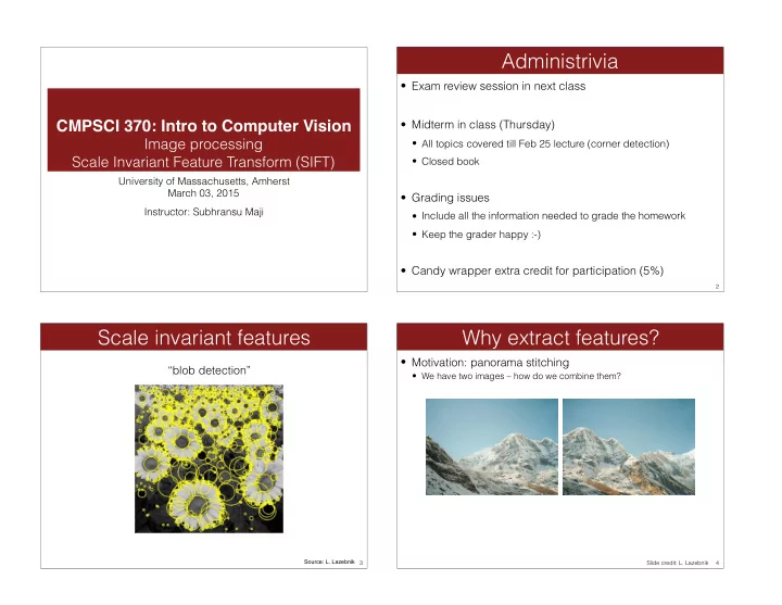
Scale invariant features Why extract features? • Motivation: panorama stitching “blob detection” • We have two images – how do we combine them? Source: L. Lazebnik 3 Slide credit: L. Lazebnik 4

  2. Why extract features? Why extract features? • Motivation: panorama stitching • Motivation: panorama stitching • We have two images – how do we combine them? • We have two images – how do we combine them? Step 1: extract features Step 1: extract features Step 2: match features Step 2: match features Step 3: align images Slide credit: L. Lazebnik 5 Slide credit: L. Lazebnik 6 Feature detection with scale selection Scaling • We want to extract features with characteristic scale that matches the image transformation such as scaling and translation (a.k.a. covariance) Corner All points will be classified as Matching regions across scales edges Corner detection is sensitive to the image scale! Source: L. Lazebnik Source: L. Lazebnik 7 8

  3. Blob detection: basic idea Blob detection: basic idea • Find maxima and minima of blob filter response in space Convolve the image with a “blob filter” at multiple scales minima and scale • Look for extrema (maxima or minima) of filter response in the resulting scale space • This will give us a scale and space covariant detector = * maxima Source: L. Lazebnik Source: N. Snavely 9 10 Blob filter Recall: sharpening filter I = blurry ( I ) + sharp ( I ) sharp ( I ) = I − blurry ( I ) Laplacian of Gaussian: Circularly symmetric operator for blob detection in 2D = I ∗ e − I ∗ g σ = I ∗ ( e − g σ ) 2 2 g g ∂ ∂ 2 g ∇ = + unit impulse 2 2 x y Gaussian Laplacian of Gaussian ∂ ∂ Source: L. Lazebnik 11 12

  4. Recall: edge detection Edge detection using a Laplacian signal Edge f f Second derivative 
 2 d edge filter, e.g. of Gaussian 
 g g Derivative of a (Laplacian) 2 dx Gaussian 2 d edge response Edge = zero crossing 
 f g ∗ f*g of second derivative 2 dx Source: S. Seitz Source: S. Seitz 13 14 From edges to blobs Scale selection • edge = ripple • We want to find the characteristic scale of the blob by convolving it with Laplacians at several scales and looking • blob = superposition of two ripples for the maximum response • However, Laplacian response decays as scale increases: maximum Spatial selection : the magnitude of the Laplacian 
 response will achieve a maximum at the center of 
 original signal 
 increasing σ the blob, provided the scale of the Laplacian is 
 (radius=8) “matched” to the scale of the blob Source: L. Lazebnik Source: L. Lazebnik 15 16

  5. Scale normalization Scale normalization • The response of a derivative of Gaussian filter to a perfect • The response of a derivative of Gaussian filter to a perfect step edge decreases as σ increases step edge decreases as σ increases • To keep response the same (scale-invariant), must multiply Gaussian derivative by σ 1 • Laplacian is the second Gaussian derivative, so it must be 2 multiplied by σ 2 σ π Source: L. Lazebnik Source: L. Lazebnik 17 18 Effect of scale normalization Blob detection in 2D Laplacian of Gaussian: Circularly symmetric operator for Original signal Unnormalized Laplacian response blob detection in 2D Scale-normalized Laplacian response 2 2 g g & # ∂ ∂ 2 2 g Scale-normalized: $ ! ∇ = σ + $ ! norm 2 2 x y ∂ ∂ % " maximum Source: L. Lazebnik Source: L. Lazebnik 19 20

  6. 
 Scale selection Scale selection • At what scale does the Laplacian achieve a maximum • At what scale does the Laplacian achieve a maximum response to a binary circle of radius r? response to a binary circle of radius r? • To get maximum response, the zeros of the Laplacian have to be aligned with the circle • The Laplacian is given by (up to scale): 
 2 2 2 2 2 2 ( x y ) / 2 ( x y 2 ) e − + σ + − σ r / 2 . • Therefore, the maximum response occurs at σ = circle r r 0 Laplacian image Laplacian image Source: L. Lazebnik Source: L. Lazebnik 21 22 Characteristic scale Scale-space blob detector • We define the characteristic scale of a blob as the scale 1. Convolve image with scale-normalized Laplacian at that produces peak of Laplacian response in the blob several scales center characteristic scale T. Lindeberg (1998). "Feature detection with automatic scale selection." International Journal of Computer Vision 30 (2): pp 77--116. Source: L. Lazebnik Source: L. Lazebnik 23 24

  7. Scale-space blob detector: Example Scale-space blob detector: Example 25 26 Scale-space blob detector: Example Scale-space blob detector 1. Convolve image with scale-normalized Laplacian at several scales 2. Find maxima of squared Laplacian response in scale- space Source: L. Lazebnik Source: L. Lazebnik 27 28

  8. Efficient implementation Efficient implementation • Approximating the Laplacian with a difference of Gaussians: ( ) L 2 G ( , , x y ) G ( , , x y ) = σ σ + σ xx yy (Laplacian) DoG G x y k ( , , ) G x y ( , , ) = σ − σ (Difference of Gaussians) 2 2 2 2 2 2 ( x y ) / 2 ( x y 2 ) e − + σ + − σ Is the Laplacian separable? David G. Lowe. "Distinctive image features from scale-invariant keypoints.” IJCV 60 (2), pp. 91-110, 2004. Source: L. Lazebnik 29 30 From feature detection to description Eliminating rotation ambiguity • Scaled and rotated versions of the same neighborhood will • To assign a unique orientation to circular image windows: give rise to blobs that are related by the same transformation • Create histogram of local gradient directions in the patch • • What to do if we want to compare the appearance of these Assign canonical orientation at peak of smoothed histogram image regions? Normalization : transform these regions into same-size • circles • Problem: rotational ambiguity 2 π 0 Source: L. Lazebnik Source: L. Lazebnik 31 32

  9. From feature detection to description SIFT features • Detected features with characteristic scales and orientations: how should we represent the patches? David G. Lowe. "Distinctive image features from scale-invariant keypoints.” IJCV 60 (2), pp. 91-110, 2004. Source: L. Lazebnik Source: L. Lazebnik 33 34

Download Presentation
Download Policy: The content available on the website is offered to you 'AS IS' for your personal information and use only. It cannot be commercialized, licensed, or distributed on other websites without prior consent from the author. To download a presentation, simply click this link. If you encounter any difficulties during the download process, it's possible that the publisher has removed the file from their server.

Recommend


More recommend