
SLIDE 1
Administrivia
See
http://www.ee.columbia.edu/ stanchen/fall09/e6870/readings/project f09.html
for suggested readings and presentation guidelines for final project.
- ✁
EECS E6870: Advanced Speech Recognition 2
EECS E6870 - Speech Recognition Lecture 11
Stanley F . Chen, Michael A. Picheny and Bhuvana Ramabhadran IBM T.J. Watson Research Center Yorktown Heights, NY, USA Columbia University stanchen@us.ibm.com, picheny@us.ibm.com, bhuvana@us.ibm.com
24 November 2009
✄☎ ✆EECS E6870: Advanced Speech Recognition
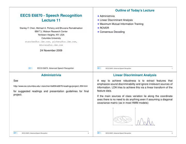
Linear Discriminant Analysis
A way to achieve robustness is to extract features that emphasize sound discriminability and ignore irrelevant sources of
- information. LDA tries to achieve this via a linear transform of the
feature data. If the main sources of class variation lie along the coordinate axes there is no need to do anything even if assuming a diagonal covariance matrix (as in most HMM models):
✝✞ ✟EECS E6870: Advanced Speech Recognition 3
Outline of Today’s Lecture
■ Administrivia ■ Linear Discriminant Analysis ■ Maximum Mutual Information Training ■ ROVER ■ Consensus Decoding
✠✡ ☛EECS E6870: Advanced Speech Recognition 1