Administrivia Mini-project 2 due April 7, in class implement - PowerPoint PPT Presentation

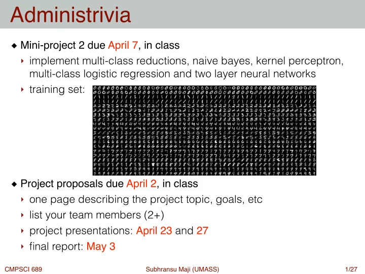
Administrivia Mini-project 2 due April 7, in class � ‣ implement multi-class reductions, naive bayes, kernel perceptron, multi-class logistic regression and two layer neural networks ‣ training set: � � � � � Project proposals due April 2, in class � ‣ one page describing the project topic, goals, etc ‣ list your team members (2+) ‣ project presentations: April 23 and 27 ‣ final report: May 3 CMPSCI 689 Subhransu Maji (UMASS) 1 /27

Kaggle https://www.kaggle.com/competitions CMPSCI 689 Subhransu Maji (UMASS) 2 /27

Kernel Methods Subhransu Maji CMPSCI 689: Machine Learning 24 March 2015 26 March 2015

Feature mapping Learn non-linear classifiers by mapping features Can we learn the XOR function with this mapping? CMPSCI 689 Subhransu Maji (UMASS) 4 /27

Quadratic feature map x = [ x 1 , x 2 , . . . , x D ] Let, � Then the quadratic feature map is defined as: � � √ √ √ φ ( x ) =[1 , 2 x 1 , 2 x 2 , . . . , 2 x D , � x 2 � 1 , x 1 x 2 , x 1 x 3 . . . , x 1 x D , � x 2 x 1 , x 2 2 , x 2 x 3 . . . , x 2 x D , � . . . , � x D x 1 , x D x 2 , x D x 3 . . . , x 2 D ] � � Contains all single and pairwise terms � There are repetitions, e.g., x 1 x 2 and x 2 x 1, but hopefully the learning algorithm can handle redundant features CMPSCI 689 Subhransu Maji (UMASS) 5 /27

Drawbacks of feature mapping Computational � ‣ Suppose training time is linear in feature dimension, quadratic feature map squares the training time Memory � ‣ Quadratic feature map squares the memory required to store the training data Statistical � ‣ Quadratic feature mapping squares the number of parameters ‣ For now lets assume that regularization will deal with overfitting CMPSCI 689 Subhransu Maji (UMASS) 6 /27

Quadratic kernel The dot product between feature maps of x and z is: � � φ ( x ) T φ ( z ) = 1 + 2 x 1 z 1 + 2 x 2 z 2 , . . . , 2 x D z D + x 2 1 z 2 1 + x 1 x 2 z 1 z 2 + . . . + x 1 x D z 1 z D + . . . � . . . + x D x 1 z D z 1 + x D x 2 z D z 2 + . . . + x 2 D z 2 D � X ! X = 1 + 2 + x i z i x i x j z i z j � i i,j � x T z + ( x T z ) 2 � � = 1 + 2 � � 2 1 + x T z � = � = K ( x , z ) quadratic kernel � Thus, we can compute φ ( x ) ᵀ φ ( z ) in almost the same time as needed to compute x ᵀ z (one extra addition and multiplication) � We will rewrite various algorithms using only dot products (or kernel evaluations), and not explicit features CMPSCI 689 Subhransu Maji (UMASS) 7 /27

Perceptron revisited Input: training data ( x 1 , y 1 ) , ( x 2 , y 2 ) , . . . , ( x n , y n ) feature map φ Perceptron training algorithm w ← [0 , . . . , 0] Initialize � for iter = 1,…,T � ‣ for i = 1,..,n � • predict according to the current model � � if w T φ ( x i ) > 0 ⇢ +1 y i = ˆ � − 1 otherwise dependence on φ � • if , no change � y i = ˆ y i • else, w ← w + y i φ ( x i ) Obtained by replacing x by φ ( x ) CMPSCI 689 Subhransu Maji (UMASS) 8 /19

Properties of the weight vector Linear algebra recap: � ‣ Let U be set of vectors in R ᴰ , i.e., U = { u 1, u 2, …, u D } and u i ∈ R ᴰ ‣ Span(U) is the set of all vectors that can be represented as ∑ ᵢ a ᵢ u ᵢ , such that a ᵢ ∈ R ‣ Null(U) is everything that is left i.e., R ᴰ \ Span(U) Perceptron representer theorem: During the run of the perceptron training algorithm, the weight vector w is always in the span of φ ( x 1 ), φ ( x 1 ), …, φ ( x D ) w = P i α i φ ( x i ) updates α i ← α i + y i i α i φ ( x i )) T φ ( z ) = P w T φ ( z ) = ( P i α i φ ( x i ) T φ ( z ) CMPSCI 689 Subhransu Maji (UMASS) 9 /27

Kernelized perceptron Input: training data ( x 1 , y 1 ) , ( x 2 , y 2 ) , . . . , ( x n , y n ) feature map φ Kernelized perceptron training algorithm α ← [0 , 0 , . . . , 0] Initialize � for iter = 1,…,T � ‣ for i = 1,..,n � • predict according to the current model � n α n φ ( x n ) T φ ( x i ) > 0 � ⇢ if P +1 y i = ˆ � − 1 otherwise � • if , no change � y i = ˆ y i • else, α i = α i + y i φ ( x ) T φ ( z ) = (1 + x T z ) p polynomial kernel of degree p CMPSCI 689 Subhransu Maji (UMASS) 10 /19

Support vector machines Kernels existed long before SVMs, but were popularized by them � Does the representer theorem hold for SVMs? � Recall that the objective function of an SVM is: � � 1 2 || w || 2 + C X max(0 , 1 − y n w T x n ) min � w n � Let, w = w k + w ? norm decomposes only w || affects classification w T w = ( w k + w ? ) T ( w k + w ? ) w T x i = ( w k + w ? ) T x i = w T k x i + w T = w T k w k + w T ? x i ? w ? = w T ≥ w T k x i k w k w ∈ Span( { x 1 , x 2 , . . . , x n } ) Hence, CMPSCI 689 Subhransu Maji (UMASS) 11 /27

Kernel k-means Initialize k centers by picking k points randomly � Repeat till convergence (or max iterations) � ‣ Assign each point to the nearest center (assignment step) k � X X || φ ( x ) − µ i || 2 arg min � S i =1 x ∈ S i � ‣ Estimate the mean of each group (update step) k � X X || φ ( x ) − µ i || 2 arg min � S i =1 x ∈ S i � 1 X φ ( x ) µ i ← Representer theorem is easy here — � | S i | x ∈ S i � � || φ ( x ) − µ i || 2 Exercise: show how to compute using dot products CMPSCI 689 Subhransu Maji (UMASS) 12 /37

What makes a kernel? A kernel is a mapping K: X x X → R � Functions that can be written as dot products are valid kernels � K ( x , z ) = φ ( x ) T φ ( z ) � K d (poly) ( x , z ) = (1 + x T z ) d Examples: polynomial kernel � � Alternate characterization of a kernel � A function K: X x X → R is a kernel if K is positive semi-definite (psd) � This property is also called as Mercer’s condition � This means that for all functions f that are squared integrable except the zero function, the following property holds: Z Z Z f ( x ) 2 d x < ∞ f ( x ) K ( x , z ) f ( z ) d z d x > 0 CMPSCI 689 Subhransu Maji (UMASS) 13 /27

Why is this characterization useful? We can prove some properties about kernels that are otherwise hard to prove � Theorem: If K 1 and K 2 are kernels, then K 1 + K 2 is also a kernel � Proof: � Z Z Z Z � f ( x ) K ( x , z ) f ( z ) d z d x = f ( x ) ( K 1 ( x , z ) + K 2 ( x , z )) f ( z ) d z d x � Z Z Z Z = f ( x ) K 1 ( x , z ) f ( z ) d z d x + f ( x ) K 2 ( x , z ) f ( z ) d z d x � ≥ 0 + 0 � More generally if K 1 , K 2 ,…, K n are kernels then ∑ᵢα i K i with α i ≥ 0, is a also a kernel � Can build new kernels by linearly combining existing kernels CMPSCI 689 Subhransu Maji (UMASS) 14 /27

Why is this characterization useful? We can show that the Gaussian function is a kernel � ‣ Also called as radial basis function (RBF) kernel − γ || x − z || 2 � � K (rbf) ( x , z ) = exp � Lets look at the classification function using a SVM with RBF kernel: � � � X f ( z ) = α i K (rbf) ( x i , z ) � i � X − γ || x i − z || 2 � � = α i exp � i � � This is similar to a two layer network with the RBF as the link function � Gaussian kernels are examples of universal kernels — they can approximate any function in the limit as training data goes to infinity CMPSCI 689 Subhransu Maji (UMASS) 15 /27

Kernels in practice Feature mapping via kernels often improves performance � MNIST digits test error: � ‣ 8.4% SVM linear ‣ 1.4% SVM RBF ‣ 1.1% SVM polynomial (d=4) 60,000 training examples http://yann.lecun.com/exdb/mnist/ CMPSCI 689 Subhransu Maji (UMASS) 16 /27

Kernels over general structures Kernels can be defined over any pair of inputs such as strings, trees and graphs! � Kernel over trees: � � K ( ) , number of common � � = subtrees � � � http://en.wikipedia.org/wiki/Tree_kernel � ‣ This can be computed efficiently using dynamic programming ‣ Can be used with SVMs, perceptrons, k-means, etc For strings number of common substrings is a kernel � Graph kernels that measure graph similarity (e.g. number of common subgraphs) have been used to predict toxicity of chemical structures CMPSCI 689 Subhransu Maji (UMASS) 17 /27

Kernels for computer vision Histogram intersection kernel between two histograms a and b � � � � � � a � b � � min (a,b) � � Introduced by Swain and Ballard 1991 to compare color histograms CMPSCI 689 Subhransu Maji (UMASS) 18 /27

Kernel classifiers tradeoffs Evaluation ¡time Non-­‑linear ¡Kernel N X h ( z ) = α i K ( x i , z ) Linear ¡Kernel i =1 h ( z ) = w T z Accuracy Linear: ¡ ¡ ¡ ¡ ¡ ¡ ¡ ¡ ¡ ¡ ¡ ¡O ¡(feature ¡dimension) ¡ Non ¡Linear: ¡ ¡ ¡O ¡( N ¡ X ¡feature ¡dimension) CMPSCI 689 Subhransu Maji (UMASS) 19 /27

Kernel classification function 0 1 N N D X X X h ( z ) = α i K ( x i , z ) = min( x ij , z j ) α i @ A i =1 i =1 j =1 CMPSCI 689 Subhransu Maji (UMASS) 20 /27

Kernel classification function 0 1 N N D X X X h ( z ) = α i K ( x i , z ) = min( x ij , z j ) α i @ A i =1 i =1 j =1 Key insight: additive property 0 1 N D X X h ( z ) = min( x ij , z j ) α i @ A i =1 j =1 N ! D X X = α i min( x ij , z j ) j =1 i =1 D N X X = h j ( z j ) h j ( z j ) = α i min( x ij , z j ) j =1 i =1 CMPSCI 689 Subhransu Maji (UMASS) 21 /27