[PPT] - 3 pictures to keep in mind 1 Tree to Excursion Trace around the PowerPoint Presentation

SLIDE 1

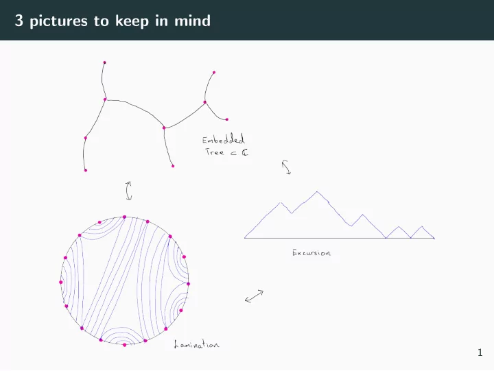
3 pictures to keep in mind

1

SLIDE 2

Tree to Excursion

Trace around the tree starting from root. Go up if seeing new edge, go down if seeing edge that’s already been seen.

2

SLIDE 3

Tree to Excursion

Trace around the tree starting from root. Go up if seeing new edge, go down if seeing edge that’s already been seen.

2

SLIDE 4

Tree to Excursion

Trace around the tree starting from root. Go up if seeing new edge, go down if seeing edge that’s already been seen.

2

SLIDE 5

Tree to Excursion

Trace around the tree starting from root. Go up if seeing new edge, go down if seeing edge that’s already been seen.

2

SLIDE 6

Tree to Excursion

Trace around the tree starting from root. Go up if seeing new edge, go down if seeing edge that’s already been seen.

2

SLIDE 7

Tree to Excursion

Trace around the tree starting from root. Go up if seeing new edge, go down if seeing edge that’s already been seen.

2

SLIDE 8

Tree to Excursion

Trace around the tree starting from root. Go up if seeing new edge, go down if seeing edge that’s already been seen.

2

SLIDE 9

Tree to Excursion

Trace around the tree starting from root. Go up if seeing new edge, go down if seeing edge that’s already been seen.

2

SLIDE 10

Tree to Excursion

Trace around the tree starting from root. Go up if seeing new edge, go down if seeing edge that’s already been seen.

2

SLIDE 11

Tree to Excursion

Trace around the tree starting from root. Go up if seeing new edge, go down if seeing edge that’s already been seen.

2

SLIDE 12

Tree to Excursion

Trace around the tree starting from root. Go up if seeing new edge, go down if seeing edge that’s already been seen.

2

SLIDE 13

Tree to Excursion

Trace around the tree starting from root. Go up if seeing new edge, go down if seeing edge that’s already been seen.

2

SLIDE 14

Tree to Excursion

Trace around the tree starting from root. Go up if seeing new edge, go down if seeing edge that’s already been seen.

2

SLIDE 15

Tree to Excursion

Trace around the tree starting from root. Go up if seeing new edge, go down if seeing edge that’s already been seen.

2

SLIDE 16

Tree to Excursion

Trace around the tree starting from root. Go up if seeing new edge, go down if seeing edge that’s already been seen.

2

SLIDE 17

Tree to Excursion

Trace around the tree starting from root. Go up if seeing new edge, go down if seeing edge that’s already been seen.

2

SLIDE 18

Tree to Excursion

Trace around the tree starting from root. Go up if seeing new edge, go down if seeing edge that’s already been seen.

2

SLIDE 19

Excursion to Tree

3

SLIDE 20

Excursion to Tree

3

SLIDE 21

Excursion to Tree

3

SLIDE 22

Excursion to Tree

3

SLIDE 23

Excursion to Tree

3

SLIDE 24

Excursion to Tree

3

SLIDE 25

Excursion to Lamination

x ∼ y ⇐ ⇒ inf

[x,y] ❡ = ❡(x) = ❡(y) 4

SLIDE 26

Excursion to Lamination

x ∼ y ⇐ ⇒ inf

[x,y] ❡ = ❡(x) = ❡(y) 4

SLIDE 27

Excursion to Lamination

x ∼ y ⇐ ⇒ inf

[x,y] ❡ = ❡(x) = ❡(y) 4

SLIDE 28

Theorem Statement

Let fn : D∗ → C be the solution to the welding problem for a uniformly random plane tree. Then as n → ∞, fn converges in distribution (w.r.t uniform convergence on ∂D) to a random map f .

5

SLIDE 29

Proof Sketch

Convergence ←Equicontinuity/Tightness ←Estimate diam(f (arc)) ≈Show that each edge is small ←Find lots of thick annuli seperating edge from infinity

6

SLIDE 30

Proof Sketch

Need to find lots of thick annuli to bound diamater of f (arc). Create annuli by joining points by geodesics (red).

7

SLIDE 31

Proof Sketch

Need to find lots of thick annuli to bound diamater of f (arc). Create annuli by joining points by geodesics (red).

7

SLIDE 32

Proof Sketch

Need to find lots of thick annuli to bound diamater of f (arc). Create annuli by joining points by geodesics (red).

7

SLIDE 33

Proof Sketch

Need to find lots of thick annuli to bound diamater of f (arc). Create annuli by joining points by geodesics (red).

7

SLIDE 34

Wishlist to make thick annuli

Conditions to ensure annulus is thick after welding?

8

SLIDE 35

Wishlist to make thick annuli

1. Need bounded number of rectangles.

9

SLIDE 36

Wishlist to make thick annuli

2. Need bounded geometry for rectangles.

9

SLIDE 37

Wishlist to make thick annuli

3. Need to know something about the welding map.

9

SLIDE 38

How to ensure that rectangle is still thick after welding

3. Need to know something about the equivalence relation.

If we can control the quality of the equivalence relation on a large subset of the edge then we get control on the modulus.

10

SLIDE 39

How to ensure that rectangle is still thick after welding

If we can control the quality of the equivalence relation on a large subset of the edge then we get control on the modulus. It’s not enough that the sets on each side are large. The equivalence relation should also behave nicely.

11

SLIDE 40

How to ensure that rectangle is still thick after welding

If we can control the quality of the equivalence relation on a large subset of the edge then we get control on the modulus. It’s not enough that the sets on each side are large. The equivalence relation should also behave nicely.

11

SLIDE 41

How to ensure that rectangle is still thick after welding

If we can control the quality of the equivalence relation on a large subset of the edge then we get control on the modulus. It’s not enough that the sets on each side are large. The equivalence relation should also behave nicely.

11

SLIDE 42

Modulus and Gluing of rectangles

Lemma We have L inf

µ−,µ+ E(µ−) + E(µ+).

µ− ranges over probability measures on I − ∩ supp(∼)
µ+ ranges over probability measures on I + ∩ supp(∼)
µ− and µ+ must be be equivalent with respect to ∼.
Energy:

E(µ) =

log

1 |x − y|dµ(x)dµ(y).

12

SLIDE 43

How to use this lemma for our problem:

Consider a toy model where we glue two squares together using the equivalence relation from a random excursion. What should we take for µ− and µ+?

13

SLIDE 44

How to use this lemma for our problem:

Consider a toy model where we glue two squares together using the equivalence relation from a random excursion. What should we take for µ− and µ+? Notice that the support of ∼ is exactly the images of the left sided and right sided inverse map of the excursion ❡ on [0, ❡(1/2)].

13

SLIDE 45

How to use this lemma for our problem:

Consider a toy model where we glue two squares together using the equivalence relation from a random excursion. What should we take for µ− and µ+? Notice that the support of ∼ is exactly the images of the left-sided and right-sided inverse map of the excursion ❡ on [0, ❡(1/2)].

13

SLIDE 46

How to use this lemma for our problem:

Thus we should take µ−, µ+ to be pullback of Lebesgue measure

n [0, ❡(1/2)] via ❡.

This demonstrates that the modulus L is controlled by the H¨

lder

regularity of ❡.

13

SLIDE 47

Wishlist to make thick annuli

To get thick annuli, want

1. Bounded number of rectangles
2. Bounded geometry rectangles
3. Control over ∼ on interface ( = regularity of excursion)

14

SLIDE 48

Finding lots of thick annuli

Now want to find lots of configurations that satisfy the conditions

f our list.

15

SLIDE 49

How to construct the annuli

Fix λ > 1. Start with large finite tree T with the graph distance. Let Xk be the points on T which are distance λk from the root. Join these points with geodesics in the complement of the tree.

16

SLIDE 50

How to construct the annuli

Fix λ > 1. Start with large finite tree T with the graph distance. Let Xk be the points on T which are distance λk from the root. Join these points with geodesics in the complement of the tree.

16

SLIDE 51

How to construct the annuli

Fix λ > 1. Start with large finite tree T with the graph distance. Let Xk be the points on T which are distance λk from the root. Join these points with geodesics in the complement of the tree.

16

SLIDE 52

How to construct the annuli

Fix λ > 1. Start with large finite tree T with the graph distance. Let Xk be the points on T which are distance λk from the root. Join these points with geodesics in the complement of the tree.

16

SLIDE 53

How to construct the annuli

Fix λ > 1. Start with large finite tree T with the graph distance. Let Xk be the points on T which are distance λk from the root. Join these points with geodesics in the complement of the tree.

16

SLIDE 54

How to construct the annuli

Fix λ > 1. Start with large finite tree T with the graph distance. Let Xk be the points on T which are distance λk from the root. Join these points with geodesics in the complement of the tree.

16

SLIDE 55

How to construct the annuli

Fix λ > 1. Start with large finite tree T with the graph distance. Let Xk be the points on T which are distance λk from the root. Join these points with geodesics in the complement of the tree.

16

SLIDE 56

How to construct the annuli

Fix λ > 1. Start with large finite tree T with the graph distance. Let Xk be the points on T which are distance λk from the root. Join these points with geodesics in the complement of the tree.

16

SLIDE 57

Rest of the proof

Analyze this exploration process via excursion picture, show

that w.h.p. on most scales k the list of conditions is satisfied.

Borel-Cantelli + Union bound =

⇒ H¨

lder equicontinuity of

welding map

Uniqueness of limit from Jones-Smirnov removability theorem.

17

SLIDE 58