
SLIDE 1
2017-07-29 1
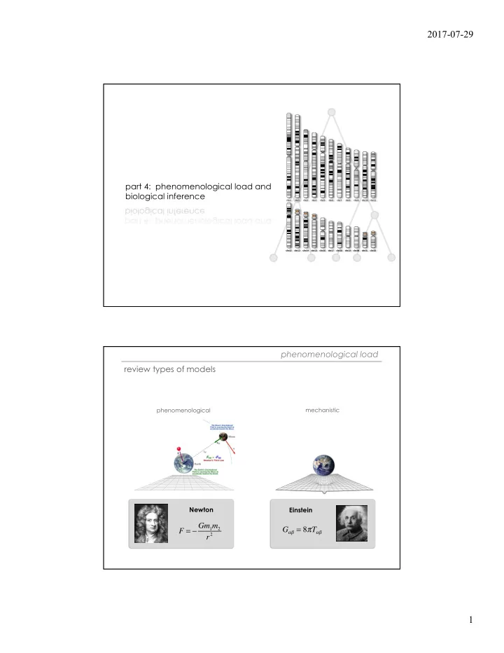
part 4: phenomenological load and biological inference phenomenological load review types of models
phenomenological mechanistic
Newton
F = − Gm1m2 r2
Einstein
Gαβ = 8πTαβ
2017-07-29 part 4: phenomenological load and biological inference - - PDF document
2017-07-29 part 4: phenomenological load and biological inference phenomenological load review types of models phenomenological mechanistic Newton Einstein F = Gm 1 m 2 G = 8 T r 2 1 2017-07-29 phenomenological load
2017-07-29 1
part 4: phenomenological load and biological inference phenomenological load review types of models
phenomenological mechanistic
Newton
F = − Gm1m2 r2
Einstein
Gαβ = 8πTαβ
2017-07-29 2
phenomenological load molecular evolution is process and pattern
“MutSel models” ! Pr = µijN × 1 N = µIJ if neutral µijN × 2sij 1− e
−2Nsij
if selected ⎧ ⎨ ⎪ ⎪ ⎩ ⎪ ⎪
sij = Δfij
Halpern(and(Bruno((1998)(
GTG CTG TCT CCT GCC GAC AAG ACC AAC GTC AAG GCC GCC TGG GGC AAG GTT GGC GCG CAC ... ... ... G.C ... ... ... T.. ..T ... ... ... ... ... ... ... ... ... .GC A.. ... ... ... ..C ..T ... ... ... ... A.. ... A.T ... ... .AA ... A.C ... AGC ... ... ..C ... G.A .AT ... ..A ... ... A.. ... AA. TG. ... ..G ... A.. ..T .GC ..T ... ..C ..G GA. ..T ... ... ..T C.. ..G ..A ... AT. ... ..T ... ..G ..A .GC ... GCT GGC GAG TAT GGT GCG GAG GCC CTG GAG AGG ATG TTC CTG TCC TTC CCC ACC ACC AAG ... ..A .CT ... ..C ..A ... ..T ... ... ... ... ... ... AG. ... ... ... ... ... .G. ... ... ... ..C ..C ... ... G.. ... ... ... ... T.. GG. ... ... ... ... ... .G. ..T ..A ... ..C .A. ... ... ..A C.. ... ... ... GCT G.. ... ... ... ... ... ..C ..T .CC ..C .CA ..T ..A ..T ..T .CC ..A .CC ... ..C ... ... ... ..T ... ..A ACC TAC TTC CCG CAC TTC GAC CTG AGC CAC GGC TCT GCC CAG GTT AAG GGC CAC GGC AAG ... ... ... ..C ... ... ... ... ... ... ... ..G ... ... ..C ... ... ... ... G.. ... ... ... ..C ... ... ... T.C .C. ... ... ... .AG ... A.C ..A .C. ... ... ... ... ... ... T.T ... A.T ..T G.A ... .C. ... ... ... ... ..C ... .CT ... ... ... ..T ... ... ..C ... ... ... ... TC. .C. ... ..C ... ... A.C C.. ..T ..T ..T ...process pattern
GTG CTG TCT CCT GCC GAC AAG ACC AAC GTC AAG GCC GCC TGG GGC AAG GTT GGC GCG CAC ... ... ... G.C ... ... ... T.. ..T ... ... ... ... ... ... ... ... ... .GC A.. ... ... ... ..C ..T ... ... ... ... A.. ... A.T ... ... .AA ... A.C ... AGC ... ... ..C ... G.A .AT ... ..A ... ... A.. ... AA. TG. ... ..G ... A.. ..T .GC ..T ... ..C ..G GA. ..T ... ... ..T C.. ..G ..A ... AT. ... ..T ... ..G ..A .GC ...
site pattern
4
Question: Does anyone really care, at all, that site pattern No.4 occurs 33 times in my sample of 5 mammalian mt genomes?
phenomenological load
Maximum phenomenological model for sequence data: explains all variation in a particular dataset
2017-07-29 3
phenomenological load
Review phenomenological models: “The good”
“The bad”
parameters
(NOT process variability) “the ugly”
phenomenological load new concept: move phenomenological from model to parameter phenomenological load (PL): if a parameter has a mechanistic interpretation, and if the process it represents did not actually occur, then when it absorbs significant variance that parameter has taken on phenomenological load (measured via PRD*). two conditions for PL: 1. confounding of model parameters 2. underspecified model
* PRD = percent reduction of deviance, and is defined in subsequent slides
2017-07-29 4
phenomenological load codon models
Qij = if i and j differ by > 1 π j for synonymous tv. κπ j for synonymous ts. ωπ j for non-synonymous tv. ωκπ j for non-synonymous ts. ⎧ ⎨ ⎪ ⎪ ⎪ ⎩ ⎪ ⎪ ⎪
DNA sub-model:
protein level sub-model:
missing model variability:
epistasis for stability)
epistasis for function)
ΔfIle→Leu
h
ΔfIle→Lys
h
phenomenological load a different look at the issue …
true model (MT) fitted model (M0)
2017-07-29 5
P
T = X |
⌢ θT
( )
P
M0 = X |
⌢ θM0
( )
KL = P
T X |
⌢ θT
( )
X
∑
log P
T (X |
⌢ θT) P
M0 X |
⌢ θM0
( )
Kullback-Leibler divergence MT M0 KL MS
DM0 = −2 lM0 ⌢ θM0 | X,T
( )− lMS X
( )
{ }
“Deviance M0”
2017-07-29 6
MT M0 KL MS M3
Not to scale!
Percent Reduction in Deviance (PDR)
PRD = DM0 − DM3 Dpoisson
MT M0 KL MS
Hypothesis tests along THIS PATH have phenomenological load
M3
PRD
Hypothesis tests along THIS PATH have direct connection to mechanism of evolution
§ significant LRTs b/c variation is not random § interpretation is not direct about mechanism of evolution
2017-07-29 7
New Q matrix
Example double: ATG (Met) è AAA (Lys) [α parameter] Example triple: AAA (Lys) è GGG (GLY) [β parameter]
DT: Double and Triple mutations
M0 Q matrix
white: probability = 0
Is such a model warranted?
Let’s do a simulation study!
African chimpanzee bonobo gorillaprocess (MT):
simulation
real mtDNA data
heat maps: proportion of sites having a given pair of AAssimulation outcome
we need outcomes to match up
Our simulated data LOOKS LIKE the REAL DATA!
2017-07-29 8
MT KL MS
simulation for MT: MutSel with NO DT-mutations
M0 M0 +DT LRT: 100% M3 M3 +DT LRT: 97% C3 C3 +DT LRT: 47%
PRD PRD PRD
since there are NO DT-mutations, PRD is a measure
PL associated with α and β PRD with true DT process PRD for real mtDNA dataset
M0 +DT M3 +DT C3 +DT Conclusions:
and β ) carry PL
process in mtDNA in excess of PL
DT very small in the real data
2017-07-29 9
MT
Poisson for codons MS Poisson for DNA JC69 MS Poisson for amino acids MS model path for inference of process m
e l p a t h f
“ s h a l l
” p h y l
e n e t i c s model path for “deep” phylogenetics Alternative model paths:
Why should you care?
levels of PL.
that expertise as part of the modeling process.
2017-07-29 10 How can you really tell if you have learned anything relevant to the function of your protein?
experimental approaches (B. Chang, next lecture)
the computational analysis of sequence evolution