. . . . . . 0 1 p-1 0 1 p-1 All-to-one Reduction Figure 4.1 - PDF document

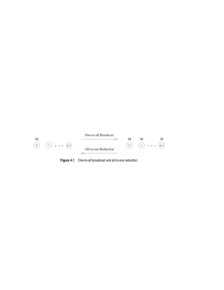
One-to-all Broadcast M M M M . . . . . . 0 1 p-1 0 1 p-1 All-to-one Reduction Figure 4.1 One-to-all broadcast and all-to-one reduction.

3 3 2 7 6 5 4 1 0 1 2 3 2 3 3 Figure 4.2 One-to-all broadcast on an eight-node ring. Node 0 is the source of the broadcast. Each message transfer step is shown by a numbered, dotted arrow from the source of the message to its destination. The number on an arrow indicates the time step during which the message is transferred.

1 1 2 7 6 5 4 3 0 1 2 3 2 1 1 Figure 4.3 Reduction on an eight-node ring with node 0 as the destination of the reduction.

All-to-one Input Vector reduction P P P P 0 1 2 3 One-to-all broadcast P P P P P 0 0 1 2 3 P P P P P 4 4 5 6 7 P Matrix P P P P 11 8 8 9 10 P P P P P 12 12 13 14 15 Output Vector Figure 4.4 One-to-all broadcast and all-to-one reduction in the multiplication of a 4 × 4 matrix with a 4 × 1 vector.

3 7 11 15 4 4 4 4 2 6 10 14 3 3 3 3 1 5 9 13 4 4 4 4 2 2 0 4 8 12 1 Figure 4.5 One-to-all broadcast on a 16-node mesh.

(110) (111) 3 6 7 (011) 2 3 (010) 2 3 3 4 5 2 1 (100) (101) 0 1 (000) (001) 3 Figure 4.6 One-to-all broadcast on a three-dimensional hypercube. The binary representations of node labels are shown in parentheses.

1 2 2 3 3 3 3 0 1 2 3 4 5 6 7 One-to-all broadcast on an eight-node tree. Figure 4.7

M -1 M -1 M p p p -1 . . . . . . . . All-to-all broadcast . M 1 M 1 M 1 M 0 M M -1 M 0 M 0 M 0 p 1 . . . . . . All-to-all reduction 0 1 p-1 0 1 p-1 Figure 4.8 All-to-all broadcast and all-to-all reduction.

1 (6) 1 (5) 1 (4) 7 6 5 4 (7) (6) (5) (4) 1 (7) 1 (3) 1st communication step (0) (1) (2) (3) 0 1 2 3 1 (0) 1 (1) 1 (2) 2 (5) 2 (4) 2 (3) 7 6 5 4 (7,6) (6,5) (5,4) (4,3) 2 (6) 2 (2) 2nd communication step (0,7) (1,0) (2,1) (3,2) 0 1 2 3 2 (7) 2 (0) 2 (1) . . . . . . 7 (0) 7 (7) 7 (6) 7 6 5 4 (7,6,5,4,3,2,1) (6,5,4,3,2,1,0) (5,4,3,2,1,0,7) (4,3,2,1,0,7,6) 7 (1) 7 (5) 7th communication step (0,7,6,5,4,3,2) (1,0,7,6,5,4,3) (2,1,0,7,6,5,4) (3,2,1,0,7,6,5) 0 1 2 3 7 (2) 7 (3) 7 (4) Figure 4.9 All-to-all broadcast on an eight-node ring. The label of each arrow shows the time step and, within parentheses, the label of the node that owned the current message being transferred before the beginning of the broadcast. The number(s) in parentheses next to each node are the labels of nodes from which data has been received prior to the current communication step. Only the first, second, and last communication steps are shown.

(6) (7) (8) (6,7,8) (6,7,8) (6,7,8) 6 7 8 6 7 8 (3) (4) (5) (3,4,5) (3,4,5) (3,4,5) 3 4 5 3 4 5 0 1 2 0 1 2 (0) (1) (2) (0,1,2) (0,1,2) (0,1,2) (a) Initial data distribution (b) Data distribution after rowwise broadcast Figure 4.10 All-to-all broadcast on a 3 × 3 mesh. The groups of nodes communicating with each other in each phase are enclosed by dotted boundaries. By the end of the second phase, all nodes get (0,1,2,3,4,5,6,7) (that is, a message from each node).

(6) (7) (6,7) (6,7) 6 7 6 7 2 3 2 3 (2) (3) (2,3) (2,3) (4) (5) 4 5 4 5 (4,5) (4,5) 0 1 0 1 (0) (1) (0,1) (0,1) (a) Initial distribution of messages (b) Distribution before the second step (0,...,7) (0,...,7) (4,5, (4,5, 6,7) 6,7) 6 7 6 7 (0,...,7) (0,...,7) (0,1, (0,1, 2 3 2 3 2,3) 2,3) (4,5, (4,5, (0,...,7) (0,...,7) 6,7) 6,7) 4 5 4 5 (0,...,7) (0,...,7) (0,1, (0,1, 0 1 0 1 2,3) 2,3) (c) Distribution before the third step (d) Final distribution of messages Figure 4.11 All-to-all broadcast on an eight-node hypercube.

Contention for a single channel by multiple messages 7 6 5 4 0 1 2 3 Figure 4.12 Contention for a channel when the communication step of Figure 4.11(c) for the hy- percube is mapped onto a ring.

(6) [6] (7) [7] (6) [6] (6+7) [6+7] 6 7 6 7 [2] [2] (2+3) (2) 2 3 (3) [3] (2+3) 2 3 [2+3] [4] 4 5 4 5 (4+5) (4) [4] (5) [5] (4+5) [4+5] [0] [0] 0 1 0 1 (0) (1) [1] (0+1) (0+1) [0+1] (a) Initial distribution of values (b) Distribution of sums before second step (4+5+6) [4+5+6] (4+5+6+7) [4+5+6+7] [0+ .. +6] [0+ .. +7] 6 7 6 7 [0+1+2] [0+1+2+3] [0+1+2+3] (0+1+ [0+1+2] 2 3 2 3 2+3) (0+1+2+3) [4] (4+5) 4 5 4 5 [4+5] (4+5) [0+1+2+3+4] [0+ .. +5] [0] (0+1+ (0+1+ 0 1 0 1 [0+1] [0] [0+1] 2+3) 2+3) (c) Distribution of sums before third step (d) Final distribution of prefix sums Figure 4.13 Computing prefix sums on an eight-node hypercube. At each node, square brackets show the local prefix sum accumulated in the result buffer and parentheses enclose the contents of the outgoing message buffer for the next step.

M -1 p . . Scatter . M 1 M 0 M 0 M 1 M -1 p . . . Gather . . . 0 1 p-1 0 1 p-1 Figure 4.14 Scatter and gather operations.

6 7 6 7 2 3 2 3 4 5 4 5 (4,5, 6,7) (0,1,2,3, (0,1, 4,5,6,7) 2,3) 0 1 0 1 (a) Initial distribution of messages (b) Distribution before the second step (6,7) (6) (7) 6 7 6 7 (2,3) (2) (3) 2 3 2 3 (4) (5) 4 5 4 5 (4,5) (0,1) (0) (1) 0 1 0 1 (c) Distribution before the third step (d) Final distribution of messages Figure 4.15 The scatter operation on an eight-node hypercube.

M 0, M 1, M p M -1,0 M M p p p p p p p -1 -1 -1, -1 -1,1 -1, -1 . . . . . . . . . . . . . . . . . . M M M -1,1 M M M 1, p p 0,1 1,1 1,0 1,1 -1 All-to-all personalized M 0,0 M M -1,0 M 0,0 M 0,1 M 0, p p 1,0 -1 communication . . . . . . 0 1 p-1 0 1 p-1 Figure 4.16 All-to-all personalized communication.

P 0 P 1 n P 2 P 3 Figure 4.17 All-to-all personalized communication in transposing a 4 × 4 matrix using four pro- cesses.

({0,5}) ({5,4}) 5 5 ({1,5}, {1,0}) ({0,4}, {0,5}) 4 4 ({2,5} ... {2,1}) ({1,4} ... {1,0}) 3 3 ({3,5} ... {3,2}) ({2,4} ... {2,1}) 2 2 ({4,5} ... {4,3}) ({3,4} ... {3,2}) 1 1 5 4 3 2 1 5 4 3 ({5,0}, ({3,0}, ({4,0}, ({2,3}, {5,1}, ({2,0}, ({1,3}, ({1,0}) {4,1}, {2,4}, ({0,3}, ({5,3}, {3,1}, {5,2}, {2,1}) {1,4}, ({4,3}) {4,2}, {2,5}, {0,4}, {3,2}) {5,3}, {5,4}) {1,5}, {4,3}) {5,4}) {2,0}, {0,5}) {1,0}) {2,1}) 0 1 2 1 2 3 4 5 ({0,1} ... {0,5}) ({1,2} ... {1,0}) 1 1 ({5,1} ... {5,4}) ({0,2} ... {0,5}) 2 2 ({4,1} ... {4,3}) ({5,2} ... {5,4}) 3 3 ({3,1}, {3,2}) ({4,2}, {4,3}) 4 4 ({2,1}) ({3,2}) 5 5 All-to-all personalized communication on a six-node ring. The label of each mes- Figure 4.18 sage is of the form { x , y } , where x is the label of the node that originally owned the mes- sage, and y is the label of the node that is the final destination of the message. The label ( { x 1 , y 1 } , { x 2 , y 2 } , . . . , { x n , y n } ) indicates a message that is formed by concatenating n indi- vidual messages.

({8,0},{8,3},{8,6}, 6 7 8 {8,1},{8,4},{8,7}, {8,2},{8,5},{8,8}) ({6,0},{6,3},{6,6}, ({7,0},{7,3},{7,6}, {6,1},{6,4},{6,7}, {7,1},{7,4},{7,7}, {6,2},{6,5},{6,8}) {7,2},{7,5},{7,8}) ({5,0},{5,3},{5,6}, 3 4 5 {5,1},{5,4},{4,7}, {5,2},{5,5},{5,8}) ({3,0},{3,3},{3,6}, ({4,0},{4,3},{4,6}, {3,1},{3,4},{3,7}, {4,1},{4,4},{4,7}, {3,2},{3,5},{3,8}) {4,2},{4,5},{4,8}) ({6,0},{6,3},{6,6}, ({6,1},{6,4},{6,7}, ({6,2},{6,5},{6,8}, {7,0},{7,3},{7,6}, {7,1},{7,4},{7,7}, {7,2},{7,5},{7,8}, {8,0},{8,3},{8,6}) {8,1},{8,4},{8,7}) {8,2},{8,5},{8,8}) 0 1 2 6 7 8 ({0,0},{0,3},{0,6}, ({1,0},{1,3},{1,6}, ({2,0},{2,3},{2,6}, {0,1},{0,4},{0,7}, ({3,1},{3,4}, ({3,2},{3,5}, {1,1},{1,4},{1,7}, {2,1},{2,4},{2,7}, {0,2},{0,5},{0,8}) {1,2},{1,5},{1,8}) {2,2},{2,5},{2,8}) {3,7},{4,1}, {3,8},{4,2}, {4,4},{4,7}, {4,5},{4,8}, {5,1},{5,,4}, {5,2},{5,5}, (a) Data distribution at the ({3,0},{3,3},{3,6}, {5,7}) {5,8}) 3 4 5 beginning of first phase {4,0},{4,3},{4,6}, {5,0},{5,3},{5,6}) ({0,1},{0,4}, ({0,2},{0,5}, {0,7},{1,1}, {0,8},{1,2}, {1,4},{1,7}, {1,5},{1,8}, {2,1},{2,4}, {2,2},{2,5}, ({0,0},{0,3},{0,6}, {2,7}) {2,8}) {1,0},{1,3},{1,6}, 0 1 2 {2,0},{2,3},{2,6}) (b) Data distribution at the beginning of second phase Figure 4.19 The distribution of messages at the beginning of each phase of all-to-all personalized communication on a 3 × 3 mesh. At the end of the second phase, node i has messages ( { 0, i } , . . . , { 8, i } ), where 0 ≤ i ≤ 8. The groups of nodes communicating together in each phase are enclosed in dotted boundaries.