Workshop 8.3a: Non-independence part 1 Murray Logan May 28, 2015 - - PDF document

workshop 8 3a non independence part 1
SMART_READER_LITE
LIVE PREVIEW

Workshop 8.3a: Non-independence part 1 Murray Logan May 28, 2015 - - PDF document

-1- Workshop 8.3a: Non-independence part 1 Murray Logan May 28, 2015 Table of contents . 1 Linear modelling assumptions 1 2 Spatial autocorrelation 9 1. Linear modelling assumptions 1.1. Linear modelling assumptions y i = 0 + 1


slide-1
SLIDE 1
  • 1-

Workshop 8.3a: Non-independence part 1

Murray Logan

May 28, 2015 .

Table of contents

1 Linear modelling assumptions 1 2 Spatial autocorrelation 9

  • 1. Linear modelling assumptions

1.1. Linear modelling assumptions

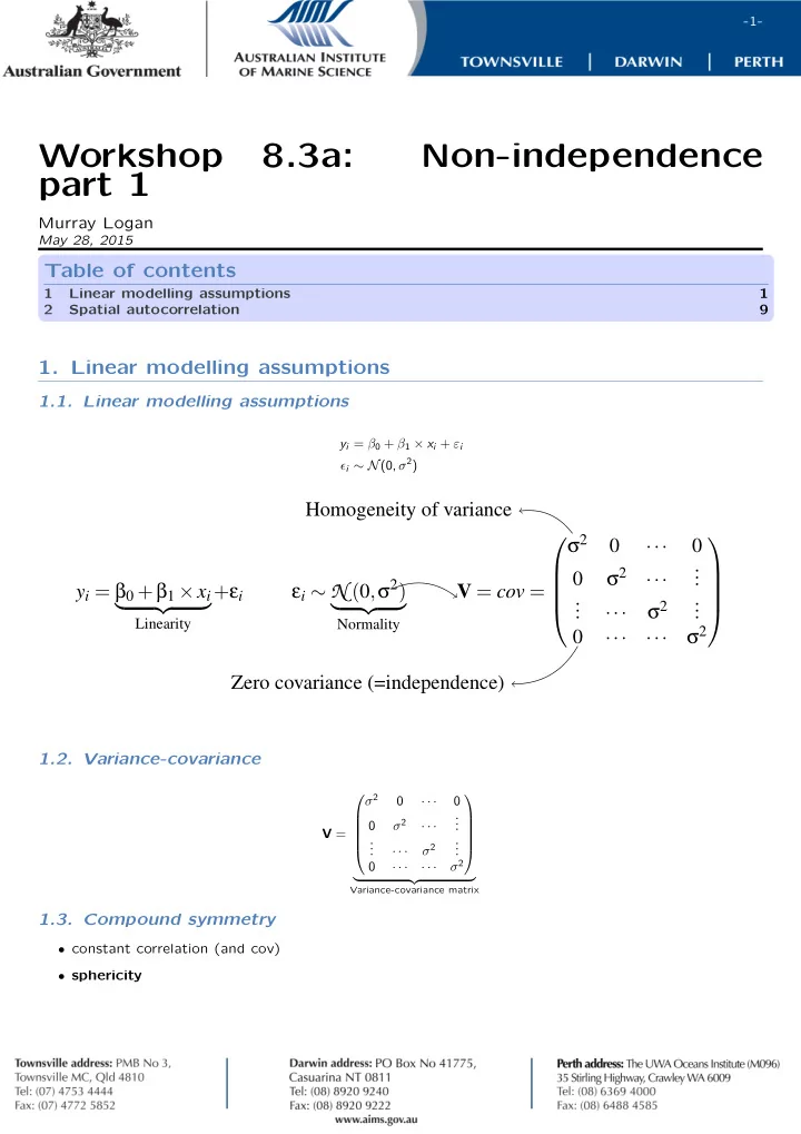
yi = β0 + β1 × xi + εi ϵi ∼ N(0, σ2)

yi = β0 +β1 ×xi

  • Linearity

+εi εi ∼ N (0,. σ2)

  • Normality

. V = cov =      . σ2 ··· σ2 ··· . . . . . . ··· σ2 . . . . ··· ··· σ2      . Homogeneity of variance . Zero covariance (=independence) .

1.2. Variance-covariance

V =       σ2 · · · σ2 · · · . . . . . . · · · σ2 . . . · · · · · · σ2      

  • Variance-covariance matrix

1.3. Compound symmetry

  • constant correlation (and cov)
  • sphericity
slide-2
SLIDE 2
  • 2-

cor(ε) =       1 ρ · · · ρ ρ 1 · · · . . . ... · · · 1 . . . ρ · · · · · · 1      

  • Correlation matrix

V =       θ + σ2 θ · · · θ θ θ + σ2 · · · . . . . . . · · · θ + σ2 . . . θ · · · · · · θ + σ2      

  • Variance-covariance matrix

1.4. Temporal autocorrelation

  • correlation dependent on proximity
  • data.t

y

20 40 60 80 100

  • 10

20 30

  • 20

40 60 80 100

  • x
  • 10

20 30

  • ● ●

1990 1995 2000 2005 2010 1990 1995 2000 2005 2010

year

1.5. Temporal autocorrelation

  • Relationship between Y and X

. . > data.t.lm <- lm(y~x, data=data.t) > par(mfrow=c(2,3)) > plot(data.t.lm, which=1:6, ask=FALSE)

slide-3
SLIDE 3
  • 3-

9.5 10.5 11.5 12.5 −20 10 20 Fitted values Residuals

  • Residuals vs Fitted

96 21 6

  • ● ●
  • −2

−1 1 2 −2 −1 1 2 Theoretical Quantiles Standardized residuals

Normal Q−Q

96 21 6

9.5 10.5 11.5 12.5 0.0 0.4 0.8 1.2 Fitted values Standardized residuals

  • Scale−Location

96 21 6

20 40 60 80 100 0.00 0.02 0.04 0.06

  • Obs. number

Cook's distance

Cook's distance

96 7 6

0.00 0.01 0.02 0.03 0.04 −2 −1 1 2 Leverage Standardized residuals

  • Cook's distance

Residuals vs Leverage

96 7 6

0.00 0.02 0.04 Leverage hii Cook's distance

  • 0.01

0.02 0.03 0.04 0.5 1 1.5 2 2.5

Cook's dist vs Leverage hii (1 −

96 7 6

1.6. Temporal autocorrelation

  • Relationship between Y and X

. . > acf(rstandard(data.t.lm))

slide-4
SLIDE 4
  • 4-

5 10 15 20 −0.2 0.0 0.2 0.4 0.6 0.8 1.0 Lag ACF

Series rstandard(data.t.lm)

1.7. Temporal autocorrelation

  • can we partial out time

. . > plot(rstandard(data.t.lm)~data.t$year)

  • 1990

1995 2000 2005 2010 −2 −1 1 2 data.t$year rstandard(data.t.lm)

slide-5
SLIDE 5
  • 5-

1.8. Temporal autocorrelation

  • can we partial out time

. . > library(car) > vif(lm(y~x+year, data=data.t))

x year 1.040037 1.040037

. . > data.t.lm1 <- lm(y~x+year, data.t)

1.9. Testing for autocorrelation

1.9.1. Residual plot

. . > par(mfrow=c(1,2)) > plot(rstandard(data.t.lm1)~fitted(data.t.lm1)) > plot(rstandard(data.t.lm1)~data.t$year)

  • −5

5 10 15 20 25 −2 −1 1 2 fitted(data.t.lm1) rstandard(data.t.lm1)

  • 1990

1995 2000 2005 2010 −2 −1 1 2 data.t$year rstandard(data.t.lm1)

1.10. Testing for autocorrelation

1.10.1. Autocorrelation (acf) plot

. . > acf(rstandard(data.t.lm1), lag=40)

slide-6
SLIDE 6
  • 6-

10 20 30 40 −0.4 0.0 0.2 0.4 0.6 0.8 1.0 Lag ACF

Series rstandard(data.t.lm1)

1.11. First order autocorrelation (AR1)

cor(ε) =       1 ρ · · · ρ|t−s| ρ 1 · · · . . . . . . · · · 1 . . . ρ|t−s| · · · · · · 1      

  • First order autoregressive correlation structure

where:

  • s and t are the times.
  • s − t is the lag

1.12. First order auto-regressive (AR1)

. . > library(nlme) > data.t.gls <- gls(y~x+year, data=data.t, method='REML') > data.t.gls1 <- gls(y~x+year, data=data.t, + correlation=corAR1(form=~year),method='REML')

1.13. First order auto-regressive (AR1)

. . > par(mfrow=c(1,2)) > plot(residuals(data.t.gls, type="normalized")~ + fitted(data.t.gls)) > plot(residuals(data.t.gls1, type="normalized")~ + fitted(data.t.gls1))

slide-7
SLIDE 7
  • 7-
  • −5

5 10 15 20 25 −2 −1 1 2 fitted(data.t.gls) residuals(data.t.gls, type = "normalized")

  • −20

−10 10 20 −2 −1 1 2 fitted(data.t.gls1) residuals(data.t.gls1, type = "normalized")

1.14. First order auto-regressive (AR1)

. . > par(mfrow=c(1,2)) > plot(residuals(data.t.gls, type="normalized")~ + data.t$x) > plot(residuals(data.t.gls1, type="normalized")~ + data.t$x)

  • 20

40 60 80 100 −2 −1 1 2 data.t$x residuals(data.t.gls, type = "normalized")

  • 20

40 60 80 100 −2 −1 1 2 data.t$x residuals(data.t.gls1, type = "normalized")

1.15. First order auto-regressive (AR1)

. . > par(mfrow=c(1,2)) > plot(residuals(data.t.gls, type="normalized")~ + data.t$year) > plot(residuals(data.t.gls1, type="normalized")~ + data.t$year)

slide-8
SLIDE 8
  • 8-
  • 1990

1995 2000 2005 2010 −2 −1 1 2 data.t$year residuals(data.t.gls, type = "normalized")

  • 1990

1995 2000 2005 2010 −2 −1 1 2 data.t$year residuals(data.t.gls1, type = "normalized")

1.16. First order auto-regressive (AR1)

. . > par(mfrow=c(1,2)) > acf(residuals(data.t.gls, type='normalized'), lag=40) > acf(residuals(data.t.gls1, type='normalized'), lag=40) 10 20 30 40 −0.4 0.0 0.2 0.4 0.6 0.8 1.0 Lag ACF

Series residuals(data.t.gls, type = "normaliz

10 20 30 40 −0.2 0.0 0.2 0.4 0.6 0.8 1.0 Lag ACF

Series residuals(data.t.gls1, type = "normaliz

1.17. First order auto-regressive (AR1)

. . > AIC(data.t.gls, data.t.gls1)

df AIC data.t.gls 4 626.3283 data.t.gls1 5 536.7467

. . > anova(data.t.gls, data.t.gls1)

Model df AIC BIC logLik Test L.Ratio p-value data.t.gls 1 4 626.3283 636.6271 -309.1642 data.t.gls1 2 5 536.7467 549.6203 -263.3734 1 vs 2 91.58158 <.0001

slide-9
SLIDE 9
  • 9-

1.18. Auto-regressive moving average (ARMA)

. . > data.t.gls2 <- update(data.t.gls, + correlation=corARMA(form=~year,p=2,q=0)) > data.t.gls3 <- update(data.t.gls, + correlation=corARMA(form=~year,p=3,q=0)) > AIC(data.t.gls, data.t.gls1, data.t.gls2, data.t.gls3)

df AIC data.t.gls 4 626.3283 data.t.gls1 5 536.7467 data.t.gls2 6 538.1032 data.t.gls3 7 538.8376

1.19. Summarize model

. . > summary(data.t.gls1)

Generalized least squares fit by REML Model: y ~ x + year Data: data.t AIC BIC logLik 536.7467 549.6203 -263.3734 Correlation Structure: ARMA(1,0) Formula: ~year Parameter estimate(s): Phi1 0.9126603 Coefficients: Value Std.Error t-value p-value (Intercept) 4388.568 1232.6129 3.560378 0.0006 x 0.028 0.0086 3.296648 0.0014 year

  • 2.195

0.6189 -3.545955 0.0006 Correlation: (Intr) x x 0.009 year -1.000 -0.010 Standardized residuals: Min Q1 Med Q3 Max

  • 1.423389

1.710551 3.377925 4.372772 6.624381 Residual standard error: 3.37516 Degrees of freedom: 100 total; 97 residual

  • 2. Spatial autocorrelation

2.1. Spatial autocorrelation

  • similar, yet dependency is 2d
  • 2d Euclidean dissimilarity
slide-10
SLIDE 10
  • 10-
  • Exponential decay

cor(ε) =       1 e−δ · · · e−δD e−δ 1 · · · . . . . . . · · · 1 . . . e−δD · · · · · · 1      

  • Exponential autoregressive correlation structure

2.2. Spatial autocorrelation

  • data.s

y

10 20 30 40 50

  • −25

−23 −21 50 100 150 200

  • 10

20 30 40 50

  • x
  • LAT

144 146 148 150

  • 50

100 150 200 −25 −23 −21

  • 144

146 148 150

  • LONG

2.3. Spatial autocorrelation

  • Spatial arrangement of Y

. . > library(sp) > coordinates(data.s) <- ~LAT+LONG > bubble(data.s,'y')

slide-11
SLIDE 11
  • 11-

y

  • 19.005

73.984 105.698 128.048 209.103

2.4. Spatial autocorrelation

  • Relationship between Y and X

. . > data.s.lm <- lm(y~x, data=data.s) > par(mfrow=c(2,3)) > plot(data.s.lm, which=1:6, ask=FALSE)

90 95 100 105 110 −100 50 100 Fitted values Residuals

  • Residuals vs Fitted

89 99 91

  • −2

−1 1 2 −2 −1 1 2 3 Theoretical Quantiles Standardized residuals

Normal Q−Q

89 99 91

90 95 100 105 110 0.0 0.5 1.0 1.5 Fitted values Standardized residuals

  • Scale−Location

89 99 91

20 40 60 80 100 0.00 0.04 0.08 0.12

  • Obs. number

Cook's distance

Cook's distance

60 50 89

0.00 0.02 0.04 0.06 −2 1 2 3 Leverage Standardized residuals

  • Cook's distance

Residuals vs Leverage

60 50 89

0.00 0.04 0.08 0.12 Leverage hii Cook's distance

  • 0.01

0.03 0.05 0.5 1 1.5 2 2.5 3

Cook's dist vs Leverage hii (1 −

60 50 89

2.5. Detecting spatial autocorrelation

  • bubble plot
  • semi-variogram
slide-12
SLIDE 12
  • 12-

2.6. Bubble plot

. . > data.s$Resid <- rstandard(data.s.lm) > library(sp) > #coordinates(data.s) <- ~LAT+LONG > bubble(data.s,'Resid')

Resid

  • −2.075

−0.623 0.099 0.668 2.718

2.7. Semi-variogram

  • semivariance = similarity (of residuals) between pairs at specific distances
  • distances ‘binned’ according to distance and orientation (N)
  • α

Lag (distance)=40 Lag tolerance=5 α tolerance=22.5

slide-13
SLIDE 13
  • 13-

2.8. Semi-variogram

  • 0.0

0.5 1.0 1.5 2.0 2.5 3.0

Distance

0.0 0.2 0.4 0.6 0.8 1.0 1.2

Semivariogram

Sill Range Uncorrelated points Correlated points Nugget

2.9. Semi-variogram

. > library(nlme) > data.s.gls <- gls(y~x, data.s, method='REML') > plot(nlme:::Variogram(data.s.gls, form=~LAT+LONG, + resType="normalized"))

slide-14
SLIDE 14
  • 14-

Distance Semivariogram

0.2 0.4 0.6 0.8 1.0 1.2 1 2 3 4 5

  • 2.10. Semi-variogram

. . > library(gstat) > plot(variogram(residuals(data.s.gls,"normalized")~1, + data=data.s, cutoff=6))

distance semivariance

0.2 0.4 0.6 0.8 1.0 1.2 1 2 3 4 5

slide-15
SLIDE 15
  • 15-

2.11. Semi-variogram

. . > library(gstat) > plot(variogram(residuals(data.s.gls,"normalized")~1, + data=data.s, cutoff=6,alpha=c(0,45,90,135)))

distance semivariance

0.5 1.0 1.5 2.0 2.5 1 2 3 4 5

  • 45
  • 90

1 2 3 4 5 0.5 1.0 1.5 2.0 2.5

  • 135

2.12. Accommodating spatial autocorrelation

Correlation function Correlation structure Description corExp(form= lat+long) Exponential Φ = 1 − e−D/ρ varGaus(form= lat+long) Gaussian Φ = 1 − e−(D/ρ)2 varLin(form= lat+long) Linear Φ = 1 − (1 − D/ρ)I(d < ρ) varRatio(form= lat+long) Rational quadratic Φ = (d/ρ)2/(1 + (d/ρ)2) varSpher(form= lat+long) Spherical Φ = 1 − (1 − 1.5(d/ρ) + 0.5(d/ρ)3)I(d < ρ)

0.0 1.0 2.0 3.0

Distance

0.0 0.2 0.4 0.6 0.8 1.0

Semivariogram Exponential

0.0 1.0 2.0 3.0

Distance

0.0 0.2 0.4 0.6 0.8 1.0

Semivariogram Gaussian

0.0 1.0 2.0 3.0

Distance

0.0 0.2 0.4 0.6 0.8 1.0

Semivariogram Linear

0.0 1.0 2.0 3.0

Distance

0.0 0.2 0.4 0.6 0.8 1.0

Semivariogram Rational quadratic

0.0 1.0 2.0 3.0

Distance

0.0 0.2 0.4 0.6 0.8 1.0

Semivariogram Spherical

slide-16
SLIDE 16
  • 16-

2.13. Accommodating spatial autocorrelation

. . > data.s.glsExp <- update(data.s.gls, + correlation=corExp(form=~LAT+LONG, nugget=TRUE)) > data.s.glsGaus <- update(data.s.gls, + correlation=corGaus(form=~LAT+LONG, nugget=TRUE)) > #data.s.glsLin <- update(data.s/gls, > # correlation=corLin(form=~LAT+LONG, nugget=TRUE)) > data.s.glsRatio <- update(data.s.gls, + correlation=corRatio(form=~LAT+LONG, nugget=TRUE)) > data.s.glsSpher <- update(data.s.gls, + correlation=corSpher(form=~LAT+LONG, nugget=TRUE)) > > AIC(data.s.gls, data.s.glsExp, data.s.glsGaus, data.s.glsRatio, data.s.glsSpher)

df AIC data.s.gls 3 1013.9439 data.s.glsExp 5 974.3235 data.s.glsGaus 5 976.4422 data.s.glsRatio 5 974.7862 data.s.glsSpher 5 975.5244

2.14. Accommodating spatial autocorrelation

. . > plot(residuals(data.s.glsExp, type="normalized")~ + fitted(data.s.glsExp))

  • 80

90 100 110 120 −2 −1 1 2 fitted(data.s.glsExp) residuals(data.s.glsExp, type = "normalized")

2.15. Accommodating spatial autocorrelation

. . > plot(nlme:::Variogram(data.s.glsExp, form=~LAT+LONG, + resType="normalized"))

slide-17
SLIDE 17
  • 17-

Distance Semivariogram

0.2 0.4 0.6 0.8 1.0 1.2 1 2 3 4 5

  • 2.16. Summarize model

. . > summary(data.s.glsExp)

Generalized least squares fit by REML Model: y ~ x Data: data.s AIC BIC logLik 974.3235 987.2484 -482.1618 Correlation Structure: Exponential spatial correlation Formula: ~LAT + LONG Parameter estimate(s): range nugget 1.6956723 0.1280655 Coefficients: Value Std.Error t-value p-value (Intercept) 65.90018 21.824752 3.019516 0.0032 x 0.94572 0.286245 3.303886 0.0013 Correlation: (Intr) x -0.418 Standardized residuals: Min Q1 Med Q3 Max

  • 1.6019483 -0.3507695

0.1608776 0.6451751 2.1331505

slide-18
SLIDE 18
  • 18-

Residual standard error: 47.68716 Degrees of freedom: 100 total; 98 residual

. . > anova(data.s.glsExp)

  • Denom. DF: 98

numDF F-value p-value (Intercept) 1 23.45923 <.0001 x 1 10.91566 0.0013

2.17. Summarize model

. . > xs <- seq(min(data.s$x), max(data.s$x), l=100) > xmat <- model.matrix(~x, data.frame(x=xs)) > > mpred <- function(model, xmat, data.s) { + pred <- as.vector(coef(model) %*% t(xmat)) + (se<-sqrt(diag(xmat %*% vcov(model) %*% t(xmat)))) + ci <- data.frame(pred+outer(se,qt(df=nrow(data.s)-2,c(.025,.975)))) + colnames(ci) <- c('lwr','upr') + data.s.sum<-data.frame(pred, x=xs,se,ci) + data.s.sum + } > > data.s.sum<-mpred(data.s.glsExp, xmat, data.s) > data.s.sum$resid <- data.s.sum$pred+residuals(data.s.glsExp) > > library(ggplot2) > ggplot(data.s.sum, aes(y=pred, x=x))+ + geom_ribbon(aes(ymin=lwr, ymax=upr), fill='blue', alpha=0.2) + + geom_line()+geom_point(aes(y=resid)) + theme_classic()

  • 50

100 150 200 10 20 30 40 50

x pred

slide-19
SLIDE 19
  • 19-

. . > #plot(pred~x, ylim=c(min(lwr), max(upr)), data.s.sum, type="l") > #lines(lwr~x, data.s.sum) > #lines(upr~x, data.s.sum) > #points(pred+residuals(data.s.glsExp)~x, data.s.sum) > > #newdata <- data.frame(x=xs)[1,]

2.18. Summarize model

  • 50

100 150 200 10 20 30 40 50

x pred