What is System identification Using experimental data obtained from - - PowerPoint PPT Presentation

1

What is System identification

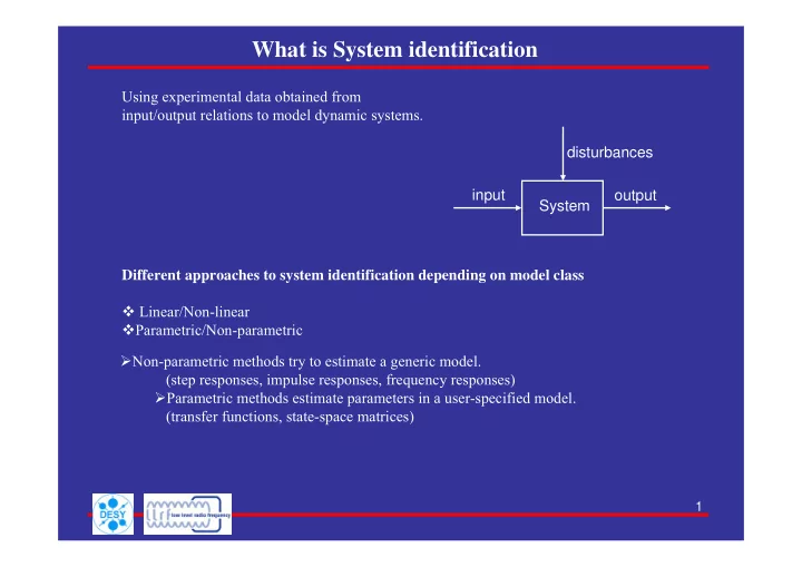
Using experimental data obtained from input/output relations to model dynamic systems. System

• utput

input disturbances Different approaches to system identification depending on model class Linear/Non-linear Parametric/Non-parametric Non-parametric methods try to estimate a generic model. (step responses, impulse responses, frequency responses) Parametric methods estimate parameters in a user-specified model. (transfer functions, state-space matrices)

2

System identification

Model validation: The model is tested in order to reveal any inadequacies. System identification includes the following steps: Experiment design: its purpose is to obtain good experimental data, and it includes the choice

• f the measured variables and of the character of the input Signals.

Selection of model structure: A suitable model structure is chosen using prior knowledge and trial and error. Choice of the criterion to fit: A suitable cost function is chosen, which reflects how well the. model fits the experimental data. Parameter estimation: An optimisation problem is solved to obtain the numerical values of the model parameters.

3

Procedure of system identification

Experimental design Data collection Data pre-filtering Model structure selection Parameter estimation Model validation Model ok? Yes No

4

Different mathematical models

Model description: Transfer functions State-space models Block diagrams (e.g. Simulink) Notation for continuous time models Complex Laplace variable ‘s’ and differential operator ‘p’

( ) ( ) ( )

t p x t t x t x = ∂ ∂ = &

Notation for discrete time models Complex z-transform variable and shift operator ‘q’

( ) ( )

k q x 1 k x = +

5

Experiments and data collection

Often good to use a two-stage approach Preliminary experiments Step/impulse response tests to get basic understanding of system dynamics Linearity, static gains, time delays constants, sampling interval Data collection for model estimation Carefully designed experiment to enable good model fit Operating point, input signal type, number of data points to collect

6

Preliminary experiments- step response

Useful for obtaining qualitative information about the system Dead time (delay) Static gain Time constants (rise time) Resonance frequency Sample time can be determined from time constants Rule-of-thumb: 4-10 sample points over the rise time

7

Design experiment for model estimation

Input signal should excite all relevant frequencies Estimated model more accurate in frequency ranges where input has high energy Pseudo-Random Binary Sequence (PRBS) is usually a good choice Trade-off in selection of signal amplitude Large amplitude gives high signal-to-noise ratio (SNR), low parameter variance Most systems are non-linear for large input amplitudes Big difference between estimation of system under closed loop control or not!

8

Collecting data

Sampling time selection and anti-alias filtering are central!

System

( )

t u

( )

t w

( )

t y

( )

t e

u

L

Y

L

( )

k u

( )

k y

+

9

Data pre-filtering

Remove: Transients needed to reach desired operating point Mean values of input and output values, i.e. work with Trends (use ‘detrend’ in MATLAB) Outliers (obvious erroneous data points)

[ ] [ ] [ ]

∑

=

− =

N 1 t

t u N 1 t u t Δu

[ ] [ ] [ ]

∑

=

− =

N 1 t

t y N 1 t y t Δy

10

General Model Structure

( )

( ) ( ) ( ) ( )

n e ,θ q H n u ,θ q G q n y

1 1 k − − −

+ =

Systems described in terms of differential equations and transfer functions. provides insight into the system physics and a compact model structure. general-linear polynomial model or the general-linear model. general-linear model structure:

+

( ) ( )

q F q B

( ) ( )

q D q C

( )

q A 1 U Y e

• are the input and output of the system.
• is zero-mean white noise, or the disturbance of the system.
• is the transfer function of the deterministic part of the system.
• is the transfer function of the stochastic part of the system.

( ) ( )

n and y n u

( )

n e

( )

,θ q G

1 −

H

11

Model structures

Model structures based on input-output: FIR Output Error Box-Jenkins ARMAX ARX Model

( )

q p ~

( ) ( )

q A q B

( ) ( )

q F q B

( ) ( )

q F q B

( )

q B

( )

q p ~

e

) ( 1 q A ) ( ) ( q A q C ) ( ) ( q D q C 1 1

[ ] [ ] ( ) ( ) [ ] [ ] ( ) [ ] ( ) [ ]

k e q p ~ k u q p ~ k

• r y

k y q D q C k u F(q) B(q) k A(q) y

e

+ = + =

( ) ( )

q A q B

Provides flexibility for system and stochastic dynamics. Simpler models that are a subset

• f the General Linear model structure.

12

Parametric Models

Each of these methods has their own advantages and disadvantages and is commonly used in real-world applications. choice of the model structure to use depends on the dynamics and the noise characteristics of the system. Using a model with more freedom or parameters is not always better as it can result in the modeling

• f nonexistent dynamics and noise characteristics.

This is where physical insight into a system is helpful. AR Model ARX Model ARMAX Model Box-Jenkins Model Output-Error Model State-Space Model

13

AR Model

process model where outputs are only dependent on previous outputs. No system inputs or disturbances are used in the modelling. class of solvable problems is limited, for signals not for systems Time series analyses, such as linear prediction coding commonly use the AR model. AR Model Structure

( )

q A 1

( )

n Y

( )

n e

14

ARX Model

Advantages: is the most efficient of the polynomial estimation methods

• > solving linear regression equations in analytic form.

unique solution, that satisfies the global minimum of the loss function. preferable, especially when the model order is high. Disadvantage: disturbances are part of the system dynamics. The transfer function of the deterministic part of the system and the transfer function of the stochastic part of the system have the same set of poles.

( )

,θ q G

1 −

( )

,θ q H

1 −

This coupling can be unrealistic. The system dynamics and stochastic dynamics of the system do not share the same set of poles all the

• time. can bias the estimation of the ARX model

However, you can reduce this disadvantage if you have a good signal-to-noise ratio.

15

ARX Model (ctnd)

Set the model order higher than the actual model order to minimize the equation error, especially when the signal-to-noise ratio is low. However, increasing the model order can change some dynamic characteristics of the model, such as the stability of the model.

+

( )

q B

( )

q A 1

( )

k u

( )

n y

( )

n e ARX Model Structure

[ ] ( ) ( ) [ ] ( ) [ ]

k e q A 1 k u q A q B k y + =

ARX (autoregressive with exogenous input)

16

ARMAX Model

includes disturbance dynamics! ARMAX models are useful when you have dominating disturbances that enter early in the process, such as at the input. i.e. a wind gust affecting an aircraft is a dominating disturbance early in the process more flexibility in the handling of disturbance modelling

+

( )

q B

( )

q C

( )

q A 1

( )

n u

( )

n y

( )

n e ARMAX Model Structure

[ ] ( ) ( ) [ ] ( ) ( ) [ ]

k e q A q C k u q A q B k y + =

ARMAX (autoregressive moving average with exogenous input)

17

Box Jenkins Model

provides a complete model with disturbance properties modelled separately from system dynamics. The Box-Jenkins model is useful when you have disturbances that enter late in the process. For example, measurement noise on the output is a disturbance late in the process. ( not output error model) Box-Jenkins Model Structure

+

( ) ( )

q F q B

( ) ( )

q D q C

( )

n u

( )

n y

( )

n e

[ ] [ ] [ ]

k e q D q C k u q F q B k y ) ( ) ( ) ( ) ( + =

18

Output Error Model

describes the system dynamics separately No parameters are used for modelling the disturbance characteristics. OE Model Structure

+

( ) ( )

q F q B

( )

n u

( )

n y

( )

n e

[ ] ( ) ( ) [ ] [ ]

k e k u q F q B k y + =

19

Space State Model

all previous methods are based on minimizing a performance function. For complex high order systems the classical methods can suffer from several problems. Find many local minima in the performance function and don’t converge to global minima. The user will need to specify complicated parameterization. They also may suffer potential problems with numerical instability and excessive computation time to execute the iterative numerical minimization methods needed. In addition, modern control methods require a state-space model of the system. For cases such as these the State-Space (SS) identification method is the appropriate model structure. When the model order is high, use an ARX model because the algorithm involved in ARX model estimation is fast and efficient when the number of data points is very large. The state-space model estimation with a large number of data points is slow and requires a large amount of memory. If you must use a state-space model, for example in modern control methods, reduce the sampling rate

• f the signal in case the sampling rate is unnecessarily high.

20

State Space (Cntd)

state vector

( )

n x

( )

n Y system output

( )

n U system input

( )

n e stochastic error system matrices. nd K: A,B,C,D, a In general, they provide a more complete representation of the system, especially for complex MIMO systems The identification procedure does not involve nonlinear optimization so the estimation reaches a solution regardless of the initial guess. parameter settings for the state-space model are simpler. You need to select only the order / states, of the model prior knowledge of the system or by analyzing the singular values of A.

( ) ( ) ( ) ( ) ( ) ( ) ( ) ( )

n e n D u n C x n Y n K e n B u n A x n x + + = + + = +1

21

Determine Parameters

Determining the delay and model order for the prediction error methods, ARMAX, BJ, and OE, is typically a trial-and-error process. The following is a useful set of steps that can lead to a suitable model. this is not the only methodology you can use, nor is this a comprehensive procedure. (1) Obtain useful information about the model order by observing the number of resonance peaks in the nonparametric frequency response function. Normally, the number of peaks in the magnitude response equals half the order of

( ) ( )

q ,F q A (2) Obtain a reasonable estimate of delay using correlation analysis and/or by testing reasonable values in a medium size ARX model. Choose the delay that provides the best model fit based on prediction error or other fit criterion. (3) Test various ARX model orders with this delay choosing those that provide the best fit. (4) Since the ARX model describes both the system dynamics and noise properties using the same set of poles, the resulting model may be unnecessarily high in order. (5)By plotting the zeros and poles and looking for cancellations you can reduce the model order.

22

Determine Parameters (Conti..)

(5) Are there additional signals? Measurements can be incorporated as extra input signals! (6) If you cannot obtain a suitable model following these steps additional physical insight into the problem might be necessary. Compensating for nonlinear sensors or actuators and handling

• f important physical non - linearities are often necessary in addition to using a ready-made

model. the higher the order of the model is, the better the model fits the data because the model has more degrees of freedom. but you need more computation time and memory choosing the model with the smallest degree of freedom, or number of parameters, if all the models fit the data well and pass the verification test.

23

Conclusion

• variety of model structures available
• choice is based upon an understanding of the system identification method and algorithm.
• system and disturbance are important
• handling a wide range of system dynamics without knowing system physics
• reduction of engineering effort
• Identification Tools (Matlab, Matrix or LabVIEW ) are available for developing, prototyping and

deploying control algorithms.

24

Matlab System Identification Tool

25

Properties of Non-linear Systems

Some properties of non-linear dynamic systems are: They do not follow the principle of superposition (linearity and homogeneity). They may have multiple isolated equilibrium points (linear systems can have only one). They may exhibit properties such as limit-cycle, bifurcation, chaos. Finite escape time: The state of an unstable nonlinear system can go to infinity in finite time. For a sinusoidal input, the output signal may contain many harmonics and sub-harmonics with various amplitudes and phase differences (a linear system's output will only contain the sinusoid at the output).

26

Analysis and Control of Non-linear Systems

There are several well-developed techniques for analyzing nonlinear feedback systems: Describing function method Phase Plane method Lyapunov stability analysis Singular Perturbation method Popov criterion (described in The Lur'e Problem below) Center manifold theorem Small-gain theorem Passivity analysis

27

Control Design of Non-linear Systems

Control design techniques for non-linear systems also exist. These can be subdivided into techniques which attempt to treat the system as a linear system in a limited range of operation and use (well-known) linear design techniques for each region: Gain Scheduling Adaptive control Those that attempt to introduce auxiliary nonlinear feedback in such a way that the system can be treated as linear for purposes of control design: Feedback linearization And Lyapunov based methods: Lyapunov Redesign Back-stepping Sliding mode control

28

Describing Function Method

procedure for analyzing Non-Linear Control problems based on quasi-linearization replacement of the non-linear system by a system that is linear except for a dependence on the amplitude of the input waveform. must be carried out for a specific family of input waveforms. An example might be the family of sine-wave inputs; in this case the system would be characterized by an SIDF or sine input describing function H (A, ω) giving the system response to an input consisting of a sine wave of amplitude A and frequency ω. (This SIDF is a generalization of the transfer function H (ω) used to characterize linear systems). Other types of describing functions that have been used are DF's for level inputs and for Gaussian noise inputs. the DF's often suffice to answer specific questions about control and stability. Example piecewise linear fact. Slope

2

s

Slope

3

s

( )

y F

y

Slope

1

s

29

Phase Plane Method

refers to graphically determining the existence of limit cycles. The Phase Plane, applicable for second order systems only, is a plot with axes being the values of the two state variables, x2 vs. x1. Vectors representing the derivatives at representative points are drawn. With enough of these arrows in place the system behaviour over the entire plane can be visualized and limit cycles can be easily identified.

( ) ( ) [ ]

2 1 2 1 2

,x x , f ,x x f 0.5 0.5

• 0.5
• 0.5

1

x

2

x

30

Lyapunov Stability

Lyapunov stability occurs in the study of dynamical systems. In simple terms, if all solutions of the dynamical system that start out near an equilibrium point xe stay near xe forever, then xe is Lyapunov

• stable. More strongly, if all solutions that start out near xe converge to xe, then xe is asymptotically s
• table. The notion of exponential stability guarantees a minimal rate of decay, i.e., an estimate of how

quickly the solutions converge. The idea of Lyapunov stability can be extended to infinite-dimensional manifolds, where it is known as Structural stability, which concerns the behaviour of different but "nearby" solutions to differential equations.

1

x

2

x

31

The Lur'e problem

Control systems have a forward path that is linear and time-invariant, and a feedback path that contains a memory-less, possibly time-varying, static non-linearity. Linear Part H(s) Non-Linear Part _ + u y The linear part can be characterized by four matrices (A,B,C,D), while the non-linear part is Φ(y) with (a sector non-linearity). by A.I. Lur'e

32

Popov criterion The sub-class of Lure's systems studied by Popov is described by:

( ) ( ) ( )

2 y φ u 1 d cx y u ξ bu Ax x − = + = = + = ξ & &

where x ∈ R n, ξ, u, y are scalars and A, b, c, d have commensurate dimensions. The non-linear element Φ: R R is a time-invariant nonlinearity belonging to open sector (0, ∞). This means that The transfer function from u to y is given by

( ) ( )

; y y ,y φ φ ≠ ∀ > =

33

Example for Popov criteria

The non-linearity is shown as a three-point characteristic, which already hosts the amplification K of the linear subsystem. KLb

• KLb

a

• a
• e

u x

( ) ( ) ( )

ω 3 j 1 ω 2 j 1 jω 1 1 + + +

( )

jω L

0.1

• 0.2
• 0.1

1 0.9 0.8 0.7 0.6 0.5 0.4 0.3 0.2

• 0.3
• 0.2
• 0.1

p

K 1 −

Popov frequency response locus Z=Lp(jω) The line g krit is tangential to the Popov frequency response locus curve and intersects the real axis at 0.1

0.1

Im Re

( )

jω L Z

p

=

krit

g

34

Popov Stability Criteria

Absolute stability The marked region in figure is called sector

( ) ( )

for e e F ke ke for e e F < ≤ ≤ > ≤ ≤

• r shorter

( )

k e e F ≤ ≤

The standard control loop is absolute stable in sector [0,k], if the closed loop only has one global asymptotic stable equilibrium for any characteristics F(e) lying in this sector

35

Popov Stability Criteria

Prerequisites:

p n ,m s a ... s a 1 s b ... s b 1 s 1 G(s)

n n 1 m m 1 p

+ < + + + + + + =

• No common zeros of numerators and denominators

F(e) is unique and at least steady in intervals . F(0)=0

p ≠

One Distinguishes the main case p=0, i.e. without integrator eigen value and the singular case IIa IIa Ib Ia Inequality Sector p Cases

m n ,...., 1 −

m n ,...., 1 −

) ( ≥ e e F ) ( ≥ ≥ e e F K ) ( ≥ ≥ e e F K ) ( > e e F

( ) ( )

) j ( G qj 1 > + ℜ ω ω

( ) ( )

K 1 ) j ( G qj 1 − > + ℜ ω ω

( ) ( )

K 1 ) j ( G qj 1 − > + ℜ ω ω

( ) ( )

) j ( G qj 1 ≥ + ℜ ω ω ω ≤

The control loop is absolute stable in the given sector , when a real number q is found for all apply on the right side of inequality. The Popov criteria is a sufficient condition for absolute stability of the control loop.

36

Popov Stability Criteria

Geometric interpretation of the Popov inequality: For the cases I b and II a, the inequality can be rewritten as follows

( ) ( ) ( ) ( ) ( ) ( ) ( ) ( ) ( ) ( ) ( )

K 1 ) j ( G q ) j ( G K 1 ) J ( G ) j ( G j q ) j ( G K 1 ) j ( G j q ) i ( G K 1 ) j ( G qj 1 − > ℑ − ℜ − > ℑ − ℜ ℜ + ℜ − > ℜ + ℜ − > + ℜ ω ω ω ω ω ω ω ω ω ω ω ω ω

One defines the modified frequency plot

( ) ( )

) j ( G j ) j ( G ) j ( Gp ω ω ω ω ℑ + ℜ =

This frequency plot is called Popov curve, so equation 1 can be represented as 1

( ) ( )

⎟ ⎠ ⎞ ⎜ ⎝ ⎛ + ℜ < ℑ K 1 ) j ( G q 1 ) j ( G

p p

ω ω

37

Example for Popov criteria

The Popov sector is defined by the line Kpe To verify Popov criteria the gradient of three-point characteristic must be smaller the calculated gradient

e a b KL

e e K p 10 =

α

1 a

10

e u

b KL a b K tan

L

= α

if this is true for the given inequality, then is idle state global asymptotic stable

10 a b KL <

38

Gain Scheduling

It is an approach to control of non-linear systems that uses a family of linear controllers, each of which provides satisfactory control for a different operating point of the system. One or more observable variables, called the scheduling variables, are used to determine what operating region the system is currently in and to enable the appropriate linear controller. For example in an aircraft flight control system, the altitude and Mach number might be the scheduling variables, with different linear controller parameters available (and automatically plugged into the controller) for various combinations of these two variables.

g

P

t

39

Adaptive Control

modifying the controller parameters to compensate slow time–varying behaviour or uncertainties. For example, as an aircraft flies, its mass will slowly decrease as a result of fuel consumption; we need a control law that adapts itself to such changing conditions. Adaptive control does not need a priori information about the bounds on these uncertain or time-varying parameters; Robust control guarantees that if the changes are within given bounds the control law need not be changed while adaptive control is precisely concerned with control law changes.

40

Adaptive Control (cntd..)

There are several broad categories of feedback adaptive control (classification can vary): Dual Adaptive Controllers Optimal Controllers. Suboptimal Dual Controllers. Nondual Adaptive Controllers. Model Reference Adaptive Controllers (MRACs) [incorporate a reference model defining desired closed loop performance] MRAC MIA Gradient Optimization MRACs [use local rule for adjusting params when performance differs from reference] Stability Optimized MRACs. Model Identification Adaptive Controllers (MIACs) [perform System identification while the system is running]. Cautious Adaptive Controllers [use current SI to modify control law, allowing for SI uncertainty]. Nonparametric Adaptive Controllers Parametric Adaptive Controllers Explicit Parameter Adaptive Controllers Implicit Parameter Adaptive Controllers

41

Feedback Linearization

• common approach used in controlling nonlinear systems.

transformation of the nonlinear system into an equivalent linear system through a change of variables and a suitable control input. Feedback linearization may be applied to nonlinear systems of the following form: The goal, then, is to develop a control input u that renders either the input-output map linear,

• r results in a linearization of the full state of the system.

( ) ( ) ( ) ( ) ( )

2 x h y 1 u x g x f x = + = &

state vector input vector

• utput vector

Existence of a state Fb control? And variable change ?

( ) ( ) y

x β x α u + =

( )

x T z = x u y

42

Pendulum example

Task: Stabilization of origin of pendulum eq.

• 1. Choose u as follows to cancel nonlinear term:

Linear system

• 2. Stabilizing fb controller

Closed loop

• 3. Re-substituting to or fb control law

v x b x x x

2 2 2 1

+ ⋅ − = = & &

( ) ( ) [ ]

cu x . b δ sin δ 1 x sin a x x x

2 2 2 1

+ − − + = = & &

( ) ( ) [ ]

c v δ sin δ x sin c a u

1

+ − + =

( ) ( ) [ ] ( )

2 2 1 1 1

x k x k c 1 δ sin δ x sin c a u + − − + ⎟ ⎠ ⎞ ⎜ ⎝ ⎛ =

2 2 1 1

x k x k v − − =

( )

2 2 1 1 2 2 1

x b k x k x x x + − = = & &

43

Sliding Mode Control

• In Control theory sliding mode control is a type of variable structure control where the dynamics of a

nonlinear system is altered via application of a high-frequency switching control. This is a state feedback control scheme where the feedback is not a continuous function of time. This control scheme involves following two steps: selection of a hypersurface or a manifold such that the system trajectory exhibits desirable behaviour when confined to this manifold. Finding feed-back gains so that the system trajectory intersects and stays on the manifold.

44

Sliding Mode Control

Switching control: Advantages Controllers with switching elements are easy to realise. The controller outputs can be restricted to a certain region of operation. Can also be used inside the region of operation to enhance the closed loop dynamics Two types of switching controllers Switching between constant values Switching between state or output dependent values Design of a switching controller therefore needs The definition of a switching condition The choice of the control law inside the areas separated by the switching law

45

Sliding Mode Control (conti..)

( ) ( )

⎩ ⎨ ⎧ < > − = y y, s 1 y y, s 1 u & &

Consider a linear system

u y= & &

The control law

ky with k u > − =

It is clear that controller is not able to stabilise the semi stable system that has two open loop eigen values of zero. The root locus plot with two branches along the imaginary axis Switching function:

( )

y my y y, s & & + =

With a scalar m>0 ,then a varibale structure controll law

46

Sliding Mode Control (conti..)

0.5 0.4

• 0.5

0.25 0.2 0.15 0.1 0.3 0.35 0.45 0.5 1

Phase plot of a closed loop system with sliding mode controller (

)

1 and m 1 y , y = = = &

47

Phase portrait with example

Consider a second order system G and h are unknown nonl. F Goal: state FB stabil the or. On the manifold s=0 motion Independent of h and g

( ) ( ) u

x g x h x x x

2 2 1

+ = = & &

x x a s

2 1 1

= + =

1

x

2

x s = ax x − = &

48

Chattering on sliding manifold

• Caused by delays not ideal would run on m.
• Region s<0 ->trajectory reverses
• Delay crossing again
• Low control accuracy.
• Power losses
• Excitation of unmodeled of dynamics
• Can result in instabilities

s < s >