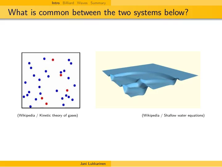
What is common between the two systems below? (Wikipedia / Kinetic - - PowerPoint PPT Presentation

Intro Billiard Waves Summary

What is common between the two systems below?

(Wikipedia / Kinetic theory of gases) (Wikipedia / Shallow water equations) Jani Lukkarinen

Intro Billiard Waves Summary

(Free) transport by particles and waves

Jani Lukkarinen 19 Jun 2018

Jani Lukkarinen

Intro Billiard Waves Summary

Classical Hamiltonian system N identical particles (hard spheres, radius r0) Reflection on the boundary In the figure, dimension d = 2 Dynamics away from the boundary determined by the Hamiltonian function H : (Rd)N × (Rd)N → R, H(q, p) =

N

• n=1

p2

n

2 + 1 2

N

• n,n′=1;n′=n

V (qn − qn′) Pair interaction potential V : Rd → R for hard spheres satisfies V (r) = g(|r|/(2r0)) , g(r) = 0 , for r > 1

Jani Lukkarinen

Intro Billiard Waves Summary

Suppose that at time t0 none of the spheres is touching each other, nor the boundary of the box: for all n′, n, |qn(t0) − qn′(t0)| > 2r0 , dist(qn(t0), ∂B) > r0 Then V (qn(t0) − qn′(t0)) = 0, and by continuity of the trajectories there must be a time-interval ε > 0 during which none of the spheres interact with each other nor with the boundary If t0 < t < t0 + ε, the Hamiltonian evolution equations read d dt qn(t) = ∇

pnH(q, p)

• q=q(t),p=p(t) = pn(t)

d dt pn(t) = −∇

qnH(q, p)

• q=q(t),p=p(t) = −
• n′=n

∇V (qn(t) − qn′(t)) = 0 ⇒ free motion = movement with constant velocity, qn(t) = qn(t0) + (t − t0)pn(t0) , pn(t) = pn(t0)

Jani Lukkarinen

Intro Billiard Waves Summary

In the limit of instantaneous collisions (infinitely hard spheres), the trajectories (q(t), p(t)) are piecewise smooth, with free motion intercepted by a finite number of collisions at which the positions are kept fixed but the velocities “jump” according to the rules of elastic collisions: If particles n = 1 and n′ = 2 collide, then (p1, p2) → (p′

1, p′ 2) with

p′

1 = p1 − [(p1 − p2) · n] n ,

p′

2 = p2 + [(p1 − p2) · n] n

where n denotes the unit vector pointing from the centre of the sphere 1 to the centre of the sphere 2

Jani Lukkarinen

Intro Billiard Waves Summary

One-particle density 6

1 Suppose that the positions and velocities are random (for simplicity)

with a probability density ρN(q, p)

2 Particles are identical ⇒ ρN is label permutation invariant

Then the average number of particles inside a volume V ⊂ Rd is given by E N

• n=1

✶{qn∈V}

• = NE[✶{q1∈V}] =
• V

dq

• Rd dp ρ1;N(q, p)

where ρ1;N denotes the first reduced one-particle density function ρ1;N(q1, p1) = N

• dq2dp2 · · · dqNdpN ρN(q, p)

Central question of transport theory How does ρ1;N evolve with time?

Jani Lukkarinen

Intro Billiard Waves Summary

How does the particle density evolve between collisions? 7

As show earlier, between collisions qn(t) = qn(t0) + (t − t0)pn(t0) , pn(t) = pn(t0) ⇒ ρN(q, p; t) = ρN(q − (t − t0)p, p; t0) Denote ft(q, p) := ρ1;N(q, p; t) ⇒ ft(q, p) = ft0(q − (t − t0)p, p) Evolution of one-particle density under free transport ∂tft(q, p) + p · ∇

qft(q, p) = 0

Jani Lukkarinen

Intro Billiard Waves Summary

Free Schr¨

• dinger evolution

8

Free Schr¨

• dinger equation ( = 1, m = 1)

i∂tψt(x) = −1 2∇2

x ψt(x)

Probability density for finding the particle = |ψt(x)|2 Can be solved explicitly by Fourier transform: Denote ψt(p) =

dx e−ip·xψt(x) and then

• ψt(p) = e−it 1

2 p2

ψ0(p)

Jani Lukkarinen

Intro Billiard Waves Summary

Wigner function and evolution of particle density 9

Wigner function of ψ W [ψ](x, v) =

• Rd

dp (2π)d eix·p ψ

v − 1

2p

∗

ψ

v + 1

2p

• Controls density both in spatial and in the Fourier variables:
• dv

(2π)d W [ψ](x, v) = |ψ(x)|2 ,

• dx W [ψ](x, v) =
• ψ(v)
• 2

Hence for free evolution, Wt(x, v) := W [ψt](x, v) = W0(x − tv, v) Free Sch¨

• dinger transport

∂tWt(x, v) + v · ∇

xWt(x, v) = 0

Jani Lukkarinen

Intro Billiard Waves Summary

General wave equations 10

Also more general wave-type evolution equations can be solved via Fourier transform:

• ψt(p) = e−itω(p)

ψ0(p) where the function ω : Rd → R is called the dispersion relation For example, standard wave equation has ω±(p) = ±|p| Large-scale transport can be solved via the Wigner function, using ∂tWt(x, k) + ∇

kω(k) · ∇ xWt(x, k) = 0

Boundary conditions still need to be properly implemented

Jani Lukkarinen

Intro Billiard Waves Summary

Summary 11

ft(q, p) := ρ1;N(q, p; t) ft controls # of particles in a phase space volume Ignore boundary and particle collisions ft(q, p) := W [ψt](q, p) ft controls spatial and Fourier densities Ignore boundary conditions and interactions ∂tft(q, p) + p · ∇

qft(q, p) = 0

Jani Lukkarinen

Intro Billiard Waves Summary

Dominant corrections ⇒ kinetic theory (rarefied gas) 12

Boltzmann–Grad scaling limit:

1 Particle radius r0 → 0 2 Assume N(2r0)2 → c0 > 0 (rarefied gas)

⇒ N → ∞

3 Assume that the particle positions and velocities are initially (t = 0)

“independently distributed”, each according to f0(x, v) Define the collision operator Cb[h](v0) = 2c0

• (Rd)3dv1dv2dv3 δ(v0 + v1 − v2 − v3)

× δ(|v0|2 + |v1|2 − |v2|2 − |v3|2) (h(v2)h(v3) − h(v0)h(v1)) Theorem (Lanford) Then there is t0 > 0 such that the r0 → 0 limit of the “one-particle distribution function” ft satisfies for 0 < t < t0 ∂tft(x, v) + v · ∇

xft(x, v) = Cb[ft(x, ·)](v)

(Scholarpedia / Boltzmann–Grad limit) Jani Lukkarinen

Intro Billiard Waves Summary

Dominant corrections ⇒ kinetic theory (waves) 13

Add a non-linear interaction term “+λ|ψt(x)|2ψt(x)” to the Schr¨

• dinger equation (nonlinear Schr¨
• dinger equation)

1 Consider a limit of weak interactions, λ → 0 2 Take tλ2 → τ, xλ2 → q 3 Consider initial data which have sufficiently fast decay of

correlations and for which the initial Wigner function has a limit Define the collision operator C[h](p1) = 2 π

• dp2dp3dp4δ(p1 + p2 − p3 − p4)

× δ(p2

1 + p2 2 − p2 3 − p2 4) (h2h3h4 + h1h3h4 − h1h2h4 − h1h2h3)

with hj = h(pj), j = 1, 2, 3, 4 ∂τfτ(q, p) + p · ∇

qfτ(q, p) = C[fτ(q, ·)](p)

(as yet unproven) Jani Lukkarinen