What is a model? A model is a representation of something. It - - PDF document

SLIDE 1

09/04/2018 1

What is a model?

A model is a representation of something. It captures not all attributes of the represented thing, but rather

• nly those that are relevant for a specific purpose.

“Confusing a model with reality would be like going to a restaurant and eat the menu”

2

like going to a restaurant and eat the menu Golomb’s Law on mathematical models

What is a good model?

• It should be expressive (an accurate representation of reality)
• It should be tractable (provide results in a bounded time)

Unfortunately, expressiveness and tractability do not get along very well

Untractability (complexity)

3

expressiveness Untractability (complexity)

Useless models (too far from reality) Useless models (too complex to be analyzed)

GOOD MODEL

Important aspects

Building a model implies:

• simplifying reality (but not too much), capturing the

features of interest;

• defining the variables that characterize the model.

4

• defining the system interface (variables exposed to the

user);

• clearly identifying the assumptions (affecting values);
• defining the metrics for evaluating the outputs of your

system and its performance.

Types of variables

• Parameters (variables you don’t want to change);
• Input variables (commands given by the user/controller)
• Design variables (variables you want to identify to apply

your control actions);

5

your control actions);

• State variables (variables describing the system state

and behavior);

• Output variables (variables you want to measure to

evaluate the performance of your method).

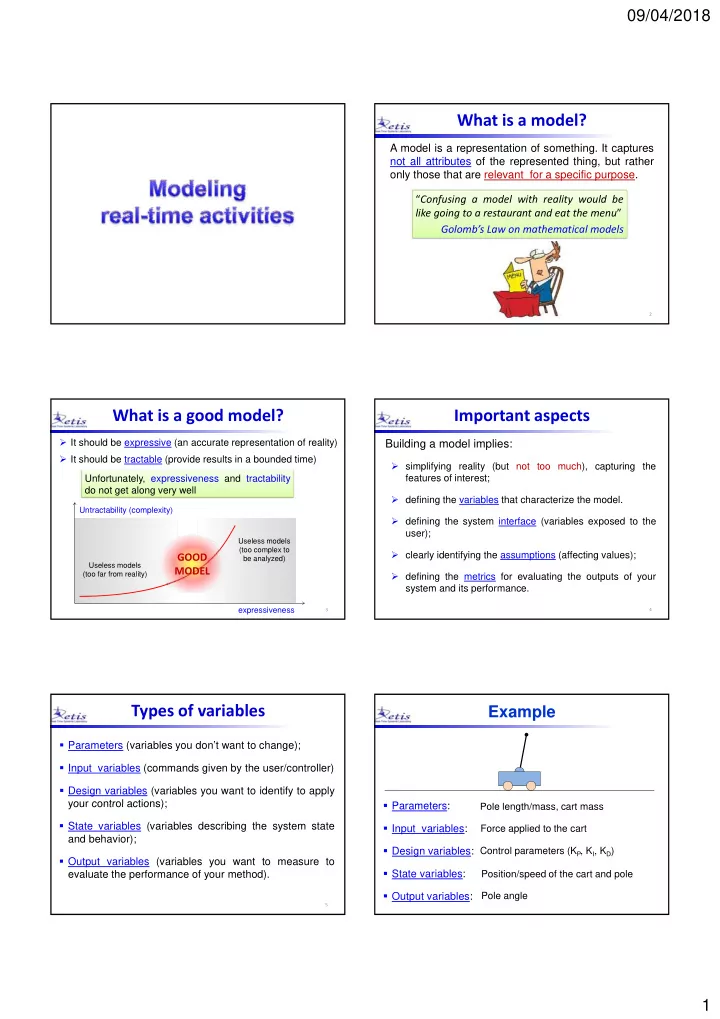
Example

• Parameters:

P l l th/ t

• Parameters:
• Input variables:
• Design variables:
• State variables:
• Output variables:

Pole length/mass, cart mass Force applied to the cart Control parameters (KP, KI, KD) Position/speed of the cart and pole Pole angle

SLIDE 2

09/04/2018 2

Elements of computation

Instruction:

It is the elementary entity of a programming language.

MOV AX, 5; MOV BX 7;

Examples in ASM X86:

7

MOV BX, 7; ADD AX, BX; int x; x = a + b; if (x > threshold) y = 1; else y = 0;

Examples in C:

Elements of computation

Function:

It is a container for a set of instructions. It may take multiple input arguments and produces a single output. a b y

8

A function can call other functions:

Elements of computation

• It is a function performing a given computational activity in a

system (e.g., sensory processing, motor control, filtering).

• It is the elementary entity managed by an operating system.
• It may have specific constraints (e g

activation time

Task:

9

• It may have specific constraints (e.g., activation time,

period, deadline, precedence relations with other tasks).

• It can communicate with other tasks by shared resources.

Resource:

It is a set of variables that can be used by tasks to store data

• r temporary results:

Elements of computation

Application:

It consists of a set of tasks interacting through a set of shared resources:

R1 R2

10

R1 R2 R3

1 2

• The

execution

• f

a task

• n

a processor is represented by a bar on a timeline.

Task execution

Task i Ci

computation time t computation time here the processor is idle

Task i

Activation time (ai) t ai si fi Ci Ri

Task important variables

Start time (si) Finishing time (fi) Computation time (Ci)

The interval fi  ai is referred to as the task response time Ri

SLIDE 3

09/04/2018 3 RTOS responsibilities

A real-time operating system is responsible for:

• Managing concurrency;
• Activating periodic tasks at the beginning of each

period (time management); p ( g )

• Deciding the execution order of tasks (scheduling);
• Solving possible timing conflicts during the access
• f shared resources (mutual exclusion);
• Manage the timely execution of asynchronous

events (interrupt handling).

Ready queue

In a concurrent system, more tasks can be simultaneously active, but only one can be in execution (running).

• An active task that is not in execution is said to be ready.
• Ready tasks are kept in a ready queue, managed by a

h d l l scheduling policy.

• The processor is assigned to the first task in the queue

through a dispatching operation.

Ready queue CPU activation dispatching termination

1 2 3

Preemption

It is a kernel mechanism that allows to suspend the execution of the running task in favor of a more important

• task. The suspended task goes back in the ready queue.

Ready queue activation dispatching termination CPU

1 2 3

preemption

• Preemption enhances concurrency and allows reducing

the response times of high priority tasks.

• It can be disabled (completely or temporarily) to ensure

the consistency of certain critical operations.

Schedule

Is a particular assignement of tasks to the processor that determines the task execution sequence: Formally, given a task set  = {1, ..., n}, a schedule is a function : R+  N that associates an integer k to each i l f i [ 1) i h h f ll i i interval of time [t, t+1) with the following meaning: k = 0 k > 0 in [t, t+1) the processor is IDLE in [t, t+1) the processor executes k

(t)

3 2

1 2 3

idle idle

Schedule

1

t t3 t4 t2 t1

• Each interval [ti, ti+1) is called a time slice.
• In time instants t1, t2, t3, t4 the processor is said to

perform a context switch.

Preemptive schedule

1 2 3

priority

3

(t)

3 2 1 2 4 6 10 12 14 8 16 18 20 2 4 6 10 12 14 8 16 18 20

SLIDE 4

09/04/2018 4

1 2 3

priority

Task states

running ready ready running running running running 3

(t)

3 2 1 2 4 6 10 12 14 8 16 18 20 2 4 6 10 12 14 8 16 18 20

dispatching wait BLOCKED signal

Task states

ACTIVE READY RUNNING activation p g preemption termination

• It is a task characterized by a timing constraint on its

response time, called deadline:

Real-Time Task

relative deadline Di



t ai si fi response time Ri di absolute deadline (di = ai + Di)

A real‐time task i is said to be feasible if it guaranteed to complete within its deadline, that is, if fi  di, o equivalently, if Ri  Di i

Slack and Lateness

t ai si fi R di Di

i

slack = d f Ri slacki = di - fi t ai si fi Ri di Di

i

lateness Li = fi - di

Performance Metrics

How do we evaluate the performance of a scheduler? For non real-time task sets:

• Average response time:

Ravg = 1/n SUM Ri

• Total finishing time:

Ftot = max(fi) – min(ri)

For real-time task sets:

• Maximum lateness:

Lmax = max(fi – di)

• No. of deadline misses:

Nmiss = SUMi H(fi – di)

• Feasibility:

F = H(Nmiss)

Tasks and jobs

A task running several times on different input data generates a sequence of instances (or jobs): ai,k ai,k+1

t

i

Ci

ai,1

Job 1

i,1 i,k i,k+1

Job k Job k+1

  

SLIDE 5

09/04/2018 5 Activation mode

• Time driven:

(periodic tasks)

A task is automatically activated by the

• perating system at predefined time instants.
• Event driven:

(aperiodic tasks)

A task is activated at the arrival of an event (by interrupt or by another task through an explicit system call).

Ci computation time

sync input

• utput

utilization factor Ci Ti Ui =

Periodic task

timer (period Ti )

• A periodic task i generates an infinite sequence of

jobs: i1, i2, …, ik (same code on different data):

Ti Ci

i ai,k ai,k+1

t Ti Ci

ai,1 = i

i (Ci , Ti , Di )

job ik

Periodic task

ai,k = i + (k1) Ti di,k = ai,k + Di

• ften

Di = Ti

task phase

 Aperiodic: ai,k+1 > ai,k  Sporadic: ai,k+1  ai,k + Ti

Aperiodic task

minimum interarrival time ai,k ai,k+1 t

i

Ci

ai,1

…

job ik

Ci Ci Application model

Using models

Task model

Definition of task/app parameters

Timing Analysis

solution

Assumptions

feasible?

NO YES Evaluation metrics

29

System to be controlled

• Sys. Req.

I/O devices

RTOS

System model Platform model RTOS model implementation

Estimating Ci is not easy

loop

? ?

• Each job operates on different data and

can take different paths.

• Even for the same data, computation time

depends on the processor state (cache, prefetch queue, number of preemptions).

# occurrencies

execution time

Ci

min

Ci

max

timer

? ?

SLIDE 6

09/04/2018 6 Predictability vs. Efficiency

# occurrencies

execution time

Ci

min

Ci

max

Ci

avg

Ci estimate

safe efficient unsafe

efficiency predictability

FIRM tasks SOFT tasks HARD tasks

Predictability vs. Efficiency

Ci

min

Ci

max

Ci

avg

Ci

Criticality

HARD task All jobs must meet their deadlines. Missing a single deadline may cause catastrophic effects on the whole system. FIRM task Missing a job deadline has not catastrophic effects on the t b t i lid t th ti f th t ti l j b system, but invalidates the execution of that particular job. SOFT task Missing a deadline is not critical. A job finishing after its deadline has still some value but causes a performance degradation. An operating system able to handle hard real-time tasks is called a hard real-time system. Typical HARD tasks – sensory acquisition – low-level control – sensory-motor planning – RT audio processing Typical FIRM tasks

Criticality

p g – RT video decoding – reading data from the keyboard – user command interpretation – message displaying – graphical activities yp Typical SOFT tasks

Jitter

t1

It is a measure of the time variation of a periodic event:

t2 t3 a1 a2 a3 a4 Absolute:

max (tk – ak) – min (tk – ak)

k k

Relative:

max | (tk – ak) – (fk-1 – ak-1) |

k

Types of Jitter

fi,1

i

Finishing‐time Jitter

fi,2 fi,3

Start‐time Jitter

si,1

i

si,2 si,3

Completion‐time Jitter (I/O Jitter)

si,1

i

si,2 si,3 fi,2 fi,1 fi,3

SLIDE 7

09/04/2018 7 Parameters summary

t

ai si fi

Ri

di Di

i

slacki

• Computation time (Ci)

ai fi di Di

Ti Ri

slacki Computation time (Ci)

• Period (Ti)
• Relative deadline (Di)
• Arrival time (ai)
• Start time (si)
• Finishing time (fi)
• Response time (Ri)
• Slack and Lateness
• Jitter

These parameters are specified by the programmer and are known off-line These parameters depend

• n

the scheduler and on the actual execution, and are known at run time.

 > 0

A control example

A positive angle  requires a positive control action u

 > 0 u > 0 u > 0  < 0

A control example

A negative angle  requires a negative control action u

u < 0  < 0 u < 0

task control(float theta0, float k) { float error; float u; float theta; while (1) {

reference angle control gain

A control task



( ) { theta = read_sensor(); error = theta – theta0; u = k * error;

• utput(u);

wait_for_next_period(); } }

sensing

u

actuation computation synchronization



task control(float theta0, float k) { float error, u, theta; while (1) { theta = read_sensor(); error = theta theta0;

u

A control task

error = theta – theta0; u = k * error;

• utput(u);

wait_for_next_period(); } }

u

task execution sensing computation actuation time task period

u t

i

Negligible delay and jitter:

u > 0 > 0

Traditional control view

 t t

 > 0  < 0  > 0  < 0 u > 0 u < 0 u < 0

SLIDE 8

09/04/2018 8

u t

i

Computation times introduce a non negligible delay:

 wrong!  

Effect of computation times

 t t

wrong! wrong!  < 0  > 0  < 0  > 0 correct  < 0  < 0 u > 0 u < 0 u < 0

u t

i

Actual situation: variable delay and jitter:

   t

Actual situation

 t t

wrong!  > 0 u < 0  < 0 u < 0 u > 0  > 0 correct correct

A robot control example

Consider a mobile robot equipped with:

• two actuated wheels;
• two proximity (US) sensors;
• a mobile (pan/tilt) camera;
• a wireless transceiver.

Goal

• Follow a path based on visual feedback;
• Avoid obstacles;
• Send complete robot status every 20 ms.

Design requirements

• Modularity:

a subsystem must be developed without knowing the details of other subsystems (team work).

• Configurability: software must be adapted to different

situations (through the use of suitable parameters) without changing the source code changing the source code.

• Portability: minimize code changes when porting the system

to different hardware platforms.

• Predictability: allow the estimation of maximum delays.
• Efficiency:
• ptimize

the use

• f

available resources (computation time, memory, energy).

Control view

• bstacle

avoidance visual‐based navigation

100 ms

• bject

recognition mot_dx mot_sx pan tilt camera US2 US1 visual tracking vehicle control

1 ms 1 ms 5 ms 10 ms 20 ms

feature extraction g

motor control motor control motor control motor control

Software View

• bstacle

avoidance visual‐based navigation

• bject

recognition

periodic task buffer mot_dx mot_sx pan tilt camera US2 US1

visual tracking vehicle control feature extraction motor control

SLIDE 9

09/04/2018 9 Software structure

INPUT OUTPUT INPUT task resource

The operating system is responsible for providing the proper mechanisms for a predictable interaction between tasks and resources.

Support for periodic tasks

Task i

while (condition) { wait_for_activation(); wait_for_next_period(); }

ready running idle active active idle idle

The IDLE state

signal wait BLOCKED Timer wait_for_next_period wake_up IDLE dispatching preemption RUNNING READY terminate activate

Design approaches

Event driven Time driven RT system RT system y(t+) x(t) polling

Environment Environment

Types of constraints

• Timing constraints

–activation, completion, jitter.

• Precedence constraints

–they impose an ordering in the execution.

• Resource constraints

–they enforce a synchronization in the access of mutually exclusive resources.

SLIDE 10

09/04/2018 10 Timing constraints

They can be explicit or implicit.

• Explicit timing constraints

They are directly included in the system specifications.

Examples –open the valve in 10 seconds –send the position within 40 ms –read the altimeter every 200 ms –acquire the camera every 20 ms

Example

Implicit timing constraints

They do not appear in the system specification, but they need to be met to satisfy the performance requirements.

t0

? Example What is the time validity of a sensory data?

Computing the yellow duration

STOP

D > Td + Tr + Tb Td = detection time Tr = reaction time Tb = braking time

Detection time:

Td = 0.6 s

Reaction time:

Tr = 0.6 s

Braking time:

Tb = v/(g) v = 50 Km/h = 14 m/s  T 2 8

Computing the yellow duration

 = 0.5 Time to stop the car from the time the yellow is turned on:  Tb = 2.8 s D > 4 s

Dashboard Controls

BRAKES human

Distribution Unit

• bstacle

v D sensor visibility

Example 2: automatic braking

condition checker

sensors emergency stop PROBLEM: Find the sampling periods of the sensors that guarantee the feasibility of the goal GOAL: If an obstacle is detected, stop the train without hitting the obstacle.

Assumptions

• Let s(Cs ,Ts) be the task devoted to sampling (Ds = Ts)
• Assume s is the task with the highest priority.
• Let Uother be the load of the other tasks

Ts

max

• bstacle not

detected in time

Ts

min

• verload

performance

Ts

load 1

SLIDE 11

09/04/2018 11 Minimum period

The system is in overload if

1  

• ther

s s

U T C

s

C T 

Hence a necessary condition The minimum period can be computed by imposing that the system is not in overload:

• ther

s s

U T   1

for the system feasibility is The maximum period can be found by a worst-case reasoning.

• ther

s s

U C T   1

min

Thus:

Worst-case reasoning

Ts

acq. task

Ts  Tb

v

• bstacle in

the field

• bstacle

detected brake pressed train stopped

D = sensor visibility

v(Ts + ) + Xb < D a = g

2 2

2 1 at vt X b  

63

g v X b   2

2

2 v = a t D g v T v

s

     2 ) (

2

    g v v D Ts  2 Tmax

g g D g v         2 ) (

2 max

64

speed

vmax v Ts

g g g v    ) (

max

g D v   2

max

65

D  = 0.5 visibility Car driving

Ts  Tb

v 60

• bstacle in

the field

• bstacle

detected brake pressed car stopped

60

Km/h

0.5 sec visibility: 50m Tmax = 0.8 sec

SLIDE 12

09/04/2018 12

Lessons learned

The farther we look, the faster we can run To go fast safely, look ahead!!! If v  vmax no feasible solution exists, no matter how fast you react!!! Don’t look away from the road for too long!!!

Example 3: contour following

v F

Goal

Move at velocity v along the surface tangent, exerting a force F < Fmax along its normal direction.

Worst-case reasoning

acq. task

v F(t-1) F(t) F(t+1) Ts

task

Ts

force not detected trajectory modified robot stopped

d

v

v = v0 e–(t/d)

Lenght covered by the robot after the contact: L = vTs + xf

d d t f

v e e v dt e v dt t v x

d

 

 /

) ( ) (      

    

 

70

L = v(Ts + d) Force on the robot tool: F = KL = Kv(Ts + d) < Fmax

(K = elastic coefficient)

Condition on the sampling period:

d s

Kv F T   

max

Tmax

      F T 

max

71

speed

vmax v0 Ts

       

d

Kv T 

max max d

K F v 

max max 

Types of constraints

• Timing constraints

– activation, completion, jitter.

• Precedence constraints

– they impose an ordering in the execution.

• Resource constraints

– they enforce a synchronization in the access of mutually exclusive resources.

SLIDE 13

09/04/2018 13 Precedence constraints

Sometimes tasks must be executed with specific precedence relations, specified through a Directed Acyclic Graph (DAG):



predecessor

1 2 3 4 5 1  2 1 4

predecessor immediate predecessor

Sample application

stereo vision processing recognition

Precedence graph

acq1 acq2 edge1 edge2 shape disp depth rec

Other task models

To refine the analysis and reduce the pessimism, a task can be modeled at a finer grain expressing:

• precedence constraints between blocks
• execution flow of internal blocks
• i l

ll l i f d

• potential parallel execution of code
• activation constraints of internal blocks
• timing constraints between internal blocks

More expressive models increase the complexity of the analysis.

Code parallelism

Fork-Join Graphs

• After a fork node, all

immediate successors must be executed (the order does not matter). fork node

• A join node is executed
• nly after all immediate

predecessors are completed. join node

Code flow

• Some task model also allows specifying activation

constraints between immediate successors as minimum interarrival times

5 8 3

SLIDE 14

09/04/2018 14 Conditional nodes

• A branch represents a conditional statement
• Only one node among all immediate successors

must be executed

switch if-then

Conditional DAGs

They include both type of semantics, allowing representing both conditional statements and parallel execution:

Nodes in conditional branches cannot have precedence relations with nodes in other branches to avoid infinite waiting times.

Types of constraints

• Timing constraints

– activation, completion, jitter.

• Precedence constraints

– they impose an ordering in the execution.

• Resource constraints

– they enforce a synchronization in the access of mutually exclusive resources.

Concurrency

Resource conflicts are caused by concurrency, that is the ability of the processor to execute more tasks at a time, by alternating their executions:

1 2 3 sequential execution parallel execution concurrent execution

Multiprogramming

Concurrency is the basic mechanism used to implement multiprogramming in multi‐user

• perating

systems (it exploits input waiting times to manage other users): Comparing sequential with concurrent executions, it seems that concurrency has no advantages:

sequential ti R1 = 4 R2 = 10 Response times

Concurrency

execution concurrent execution R3 = 15

2 4 6 10 12 14 2 4 10 12 14

R1 = 10 R2 = 15 R3 = 14

8 6 8

SLIDE 15

09/04/2018 15

If a task must wait for I/O data, concurrency allows another task to run during that interval:

sequential execution R1 = 9 R2 = 15 Response times

Concurrency and I/O

busy‐wait

1 2

2 4 6 10 12 14 2 4 10 12 14

R1 = 9 R2 = 10

8 6 8

I/O device I/O device concurrent execution

1 2

blocked

Concurrency becomes superior when managing periodic tasks at different rates (waiting times are used to execute other tasks):

sequential execution (FIFO)

Periodic tasks

(FIFO) concurrent execution (Rate Monotonic)

2 4 6 10 12 14 8 16 18 20 2 4 6 10 12 14 8 16 18 20

Hence, concurrency allows exploiting tasks inactive intervals (e.g., waiting times for input data or periodic task activation).

Concurrency: pro and cons

However, concurrency can generate conflicts when using shared resources (for example, when more tasks operate on global data).

Example of conflict

Each thread increments a counter every time an event is detected:

counter c: 10

1 2

x = counter;

global variable

x = counter;

1 2

counter 10 counter 10 11 counter 11

An event is lost!

; x = x + 1; counter = x; ; x = x + 1; counter = x;

Example 2

1 2

(x, y) global buffer It estimates the next position (x,y)

• f a moving target

It controls a missile to catch the target in (x,y) (x, y)

x = (a + b)/c; y = (a  b) /c; m1 = k1*(a*x ‐ x); m2 = k2*(a*y ‐ y); writing buffer reading buffer

x: 3 y: 5

1 2

x = 1 y = 8 It reads (3,8) which does not belong

Example 2

1 2

read(x)

3

read(y)

8

x ← 1 y ← 8

to the trajectory!

SLIDE 16

09/04/2018 16 Solution

x: 3 y: 5

1 2

x = 1 8 d (3 5)

Regulate the use of shared resources so that tasks can only access them one at the time (i.e., in mutual exclusion):

y = 8

1 2

read(x)

3

read(y)

5 reads (3,5) correctly!

x ← 1 y ← 8

blocked

1 2

Mutual exclusion is implemented by two primitives, wait(s) and signal(s), that use a system variable s, called semaphore:

Semaphores

(x, y)

x = ... y = … m1 = … x; m2 = … y; writing buffer reading buffer wait(s); signal(s); wait(s); signal(s); critical section critical section

• Each shared resourse is protected by a different

semaphore.

• s = 1  free resource,

s = 0  busy (locked) resource.

• wait(s):

if h k b bl k d f h

Semaphores

− if s == 0, the task must be blocked on a queue of the

• semaphore. The queue management policy depends
• n the OS (usually it is FIFO or priority‐based).

− else set s = 0.

• signal(s):

− if there are blocked tasks, the first in the queue is awaken (s remains 0), else set s = 1.

• If the semaphore s is initialized to 1, the pair wait(s) and

signal(s) can be used for enforcing mutual exclusion:

R

1 3

Semaphores

2

wait(s) wait(s) wait(s) signal(s) signal(s) signal(s)

s = 1 s = 0 s = 1

blocked blocked

1 2 3

• If a resource has n parallel units that can be accessed by

n tasks simultaneously, it can be protected by a semaphore initialized to n.

• wait(s):

− if s == 0 the task is blocked on the semaphore

Multi-unit resources

if s == 0, the task is blocked on the semaphore queue; − else s is decremented.

• signal(s):

− If there are blocked tasks, the first in the queue is awaken (s remains 0), else s is incremented.

s = create_sem(n) creates the semaphore structure, including a counter (s.count) initialized to n, and a queue of tasks (s.queue). wait(s) { if (s.count == 0)

Implementation notes

<block the calling task on s.queue> else s.count--; } signal(s) { if (!empty(s.queue)) <unblock the first task in s.queue> else s.count++; }

SLIDE 17

09/04/2018 17

• A semaphore initialized to 0 can be used to wait for an

event generated by another task:

Synchronization semaphores

1 2

signal(s);

calls signal(s) at the event occurrence

wait(s); signal(s);

wait(s) signal(s) blocked

1 2

priority

Problem with semaphores

• Semaphores

(when properly used) guarantee the consistency of shared global data, but introduce extra blocking delays in high priority tasks.

1 2



blocked w s w s

priority

Scheduling anomalies

T1: 3 T2: 2 T3: 2 T4: 2 T9: 9 T8: 4 T7: 4 T6: 4 T5: 4 priority

Pi > Pj  i < j

T4: 2 T5: 4

1 2 3 4 5 6 7 8 9 10 11 12 13 14

t P1 P2 P3 T1 T2 T3 T4 T9 T5 T6 T7 T8

tr = 12

Increased processors

T1: 3 T9: 9 T2: 2 T3: 2 T4: 2 T8: 4 T7: 4 T6: 4 T5: 4 P1 T1 T8 P1 P2 P3 P4

1 2 3 4 5 6 7 8 9 10 11 12 13 14

t

15

T1 T2 T3 T4 T5 T6 T7 T8 T9

tr = 15

Shorter tasks

T1: 2 T9: 8 T2: 1 T3: 1 T4: 1 T8: 3 T7: 3 T6: 3 T5: 3

1 2 3 4 5 6 7 8 9 10 11 12 13 14

t P1 P2 P3 T1 T2 T3 T4 T5 T6 T7 T8 T9

tr = 13

SLIDE 18

09/04/2018 18 Released constraints

T1: 3 T2: 2 T3: 2 T4: 2 T5: 4 T6: 4 T7: 4 T8: 4 T9: 9 P1 P2 P3

1 2 3 4 5 6 7 8 9 10 11 12 13 14 15 16

T1 T2 T3 T4 T5 T6 T7 T8 T9

tr = 16

Faster processor

1 2 1 2

double speed deadline miss

Delay: dangerous system call

A delay() may cause a delay longer than .

1  2

2 4 6 8 10 12 14 delay(2) blocked

1 2

2 4 6 8 10 12 14

A delay in a task may also increase the response time of other tasks (example for fixed priorities):

1 

4 8 12

Delay: dangerous system call

2

5 10 15 delay(1)

1 2

deadline miss 5 10 15 4 8 12

…

Lessons learned

• Tests are not enough for real-time systems
• Intuitive solutions do not always work
• Delay should not be used in real-time tasks

The safest approach:  use predictable kernel mechanisms  analyze the system to predict its behavior

Achieving predictability

• The operating system is the most important

component responsible for achieving a predictable execution.

• Concurrency control must be enforced by:
• Concurrency control must be enforced by:

 appropriate scheduling algorithms  appropriate synchronization protocols  efficient communication mechanisms  predictable interrupt handling