Visualizing Probabilities A ^ B Sample space of all possible - PDF document

Machine Learning 10-701 Tom M. Mitchell Machine Learning Department Carnegie Mellon University January 18, 2011 Today: Readings: • Bayes Rule • Estimating parameters Probability review • maximum likelihood • Bishop Ch. 1 thru 1.2.3 • max a posteriori • Bishop, Ch. 2 thru 2.2 • Andrew Moore’s online many of these slides are derived tutorial from William Cohen, Andrew Moore, Aarti Singh, Eric Xing, Carlos Guestrin. - Thanks! 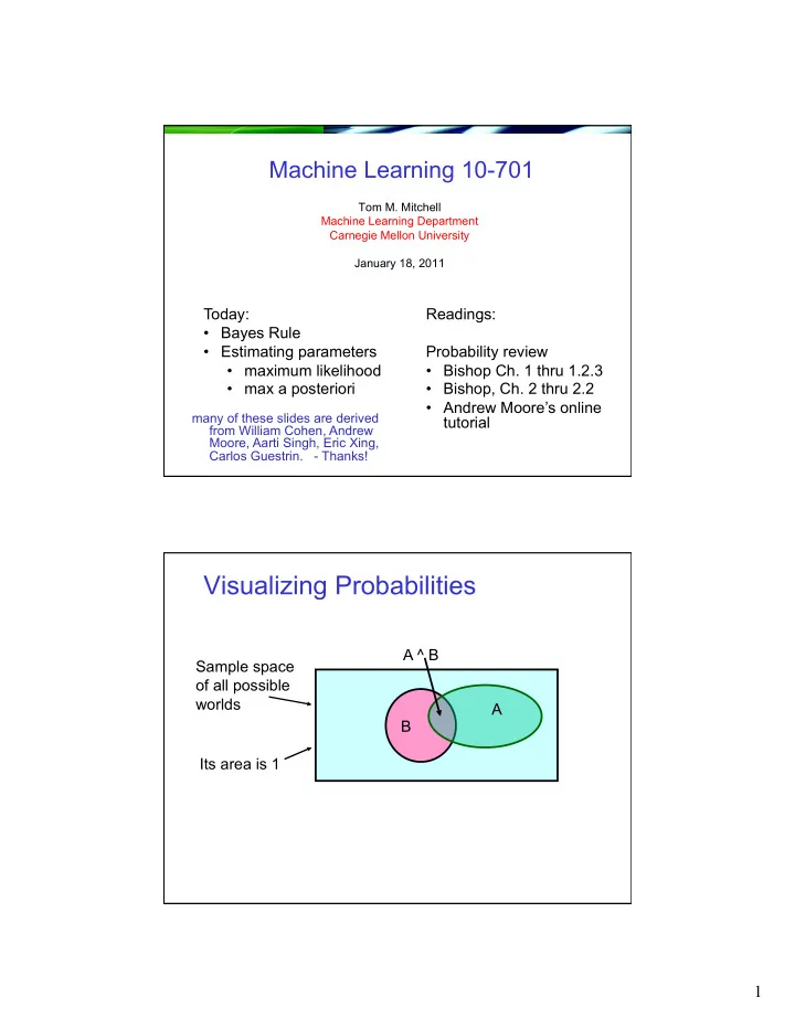Visualizing Probabilities A ^ B Sample space of all possible worlds A B Its area is 1 1

Definition of Conditional Probability P(A ^ B) P(A|B) = ----------- P(B) A B Definition of Conditional Probability P(A ^ B) P(A|B) = ----------- P(B) Corollary: The Chain Rule P(A ^ B) = P(A|B) P(B) P(C ^ A ^ B) = P(C|A ^ B) P(A|B) P(B) 2

Independent Events • Definition: two events A and B are independent if P(A ^ B)=P(A)*P(B) • Intuition: knowing A tells us nothing about the value of B (and vice versa) Bayes Rule • let’s write 2 expressions for P(A ^ B) A ^ B A B 3

P(B|A) * P(A) Bayes’ rule P(A|B) = P(B) we call P(A) the “prior” Bayes, Thomas (1763) An essay towards solving a problem in the doctrine and P(A|B) the “posterior” of chances. Philosophical Transactions of the Royal Society of London, 53:370-418 …by no means merely a curious speculation in the doctrine of chances, but necessary to be solved in order to a sure foundation for all our reasonings concerning past facts, and what is likely to be hereafter…. necessary to be considered by any that would give a clear account of the strength of analogical or inductive reasoning… Other Forms of Bayes Rule 4

Applying Bayes Rule A = you have the flu, B = you just coughed Assume: P(A) = 0.05 P(B|A) = 0.80 P(B| ~A) = 0.2 what is P(flu | cough) = P(A|B)? what does all this have to do with function approximation? 5

The Joint Distribution Example: Boolean variables A, B, C A B C Prob Recipe for making a joint 0 0 0 0.30 distribution of M variables: 0 0 1 0.05 0 1 0 0.10 0 1 1 0.05 1 0 0 0.05 1 0 1 0.10 1 1 0 0.25 1 1 1 0.10 A 0.05 0.10 0.05 0.10 0.25 0.05 C 0.10 B 0.30 [A. Moore] The Joint Distribution Example: Boolean variables A, B, C A B C Prob Recipe for making a joint 0 0 0 0.30 distribution of M variables: 0 0 1 0.05 0 1 0 0.10 1. Make a truth table listing all 0 1 1 0.05 1 0 0 0.05 combinations of values of 1 0 1 0.10 your variables (if there are 1 1 0 0.25 M Boolean variables then 1 1 1 0.10 the table will have 2 M rows). A 0.05 0.10 0.05 0.10 0.25 0.05 C 0.10 B 0.30 [A. Moore] 6

The Joint Distribution Example: Boolean variables A, B, C A B C Prob Recipe for making a joint 0 0 0 0.30 distribution of M variables: 0 0 1 0.05 0 1 0 0.10 1. Make a truth table listing all 0 1 1 0.05 1 0 0 0.05 combinations of values of 1 0 1 0.10 your variables (if there are 1 1 0 0.25 M Boolean variables then 1 1 1 0.10 the table will have 2 M rows). 2. For each combination of A 0.05 0.10 0.05 values, say how probable it 0.10 is. 0.25 0.05 C 0.10 B 0.30 [A. Moore] The Joint Distribution Example: Boolean variables A, B, C A B C Prob Recipe for making a joint 0 0 0 0.30 distribution of M variables: 0 0 1 0.05 0 1 0 0.10 1. Make a truth table listing all 0 1 1 0.05 1 0 0 0.05 combinations of values of 1 0 1 0.10 your variables (if there are 1 1 0 0.25 M Boolean variables then 1 1 1 0.10 the table will have 2 M rows). 2. For each combination of A 0.05 0.10 0.05 values, say how probable it 0.10 is. 0.25 0.05 C 3. If you subscribe to the 0.10 axioms of probability, those B 0.30 numbers must sum to 1. [A. Moore] 7

Using the Joint One you have the JD you can ask for the probability of any logical expression involving your attribute [A. Moore] Using the Joint P(Poor Male) = 0.4654 [A. Moore] 8

Using the Joint P(Poor) = 0.7604 [A. Moore] Inference with the Joint P(Male | Poor) = 0.4654 / 0.7604 = 0.612 [A. Moore] 9

Learning and the Joint Distribution Suppose we want to learn the function f: <G, H>  W Equivalently, P(W | G, H) Solution: learn joint distribution from data, calculate P(W | G, H) e.g., P(W=rich | G = female, H = 40.5- ) = [A. Moore] sounds like the solution to learning F: X  Y, or P(Y | X). Are we done? 10

[C. Guestrin] [C. Guestrin] 11

[C. Guestrin] Maximum Likelihood Estimate for Θ [C. Guestrin] 12

[C. Guestrin] [C. Guestrin] 13

[C. Guestrin] Beta prior distribution – P( θ ) [C. Guestrin] 14

Beta prior distribution – P( θ ) [C. Guestrin] [C. Guestrin] 15

[C. Guestrin] Conjugate priors [A. Singh] 16

Conjugate priors [A. Singh] Estimating Parameters • Maximum Likelihood Estimate (MLE): choose θ that maximizes probability of observed data • Maximum a Posteriori (MAP) estimate: choose θ that is most probable given prior probability and the data 17

Dirichlet distribution • number of heads in N flips of a two-sided coin – follows a binomial distribution – Beta is a good prior (conjugate prior for binomial) • what it’s not two-sided, but k-sided? – follows a multinomial distribution – Dirichlet distribution is the conjugate prior You should know • Probability basics – random variables, events, sample space, conditional probs, … – independence of random variables – Bayes rule – Joint probability distributions – calculating probabilities from the joint distribution • Estimating parameters from data – maximum likelihood estimates – maximum a posteriori estimates – distributions – binomial, Beta, Dirichlet, … – conjugate priors 18

Extra slides Expected values Given discrete random variable X, the expected value of X, written E[X] is We also can talk about the expected value of functions of X 19

Covariance Given two discrete r.v.’s X and Y, we define the covariance of X and Y as e.g., X=gender, Y=playsFootball or X=gender, Y=leftHanded Remember: 20