0 . 16 c 0 p ( a ) P ( X a ) p ( a , y - PDF document

The Questions of Our Time Life Gives You Lemmas, Make Lemma-nade! • Y is a non-negative continuous random variable • A lemma in the home or office is a good thing   Probability Density Function: f Y ( y )    E [ Y ] P ( Y y ) dy  Already knew that: E [ Y ]  0 F ( y )    E [ Y ] y f ( y ) dy    Y ( 1 F ( y )) dy    But, did you know that: 0 y  • Proof:       E [ Y ] P ( Y y ) dy ?!?      P ( Y y ) dy f ( x ) dx dy 0 Y y     No, I didn’t think so... 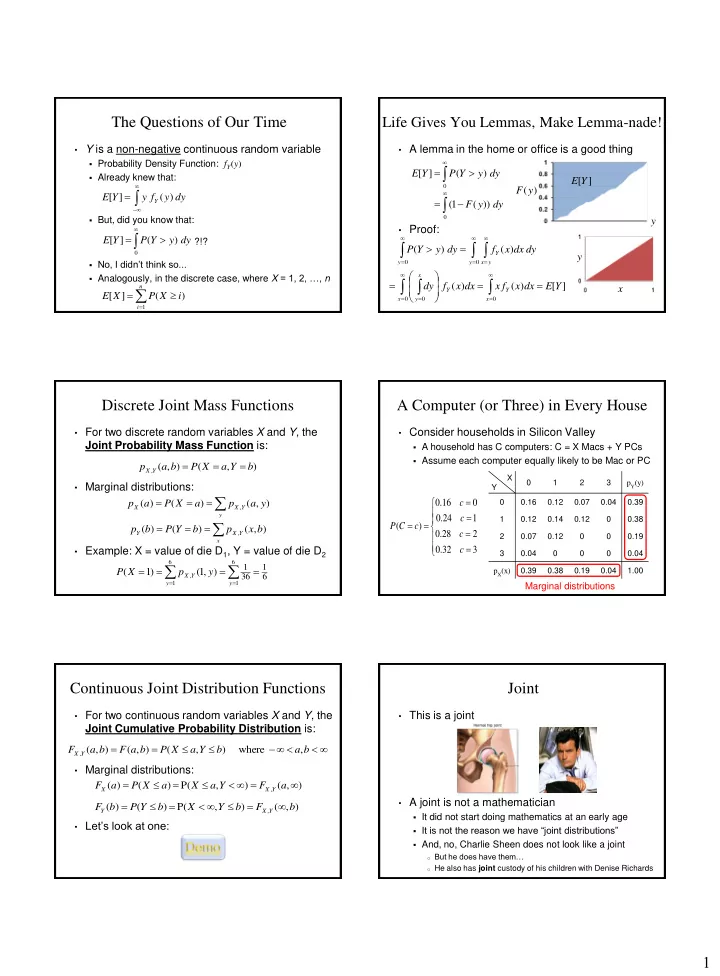y 0 y 0 x y      Analogously, in the discrete case, where X = 1, 2, …, n x         dy f ( x ) dx x f ( x ) dx E [ Y ] n   x  Y Y   E [ X ] P ( X i )      x 0 y 0 x 0  i 1 Discrete Joint Mass Functions A Computer (or Three) in Every House • For two discrete random variables X and Y , the • Consider households in Silicon Valley Joint Probability Mass Function is:  A household has C computers: C = X Macs + Y PCs  Assume each computer equally likely to be Mac or PC    p ( a , b ) P ( X a , Y b ) X , Y X 0 1 2 3 p Y (y) • Marginal distributions: Y       0 . 16 c 0 p ( a ) P ( X a ) p ( a , y ) 0 0.16 0.12 0.07 0.04 0.39 X X , Y   y  0 . 24 c 1 1 0.12 0.14 0.12 0 0.38        P ( C c ) p ( b ) P ( Y b ) p ( x , b )   0 . 28 c 2 Y X , Y 2 0.07 0.12 0 0 0.19 x    • Example: X = value of die D 1 , Y = value of die D 2 0 . 32 c 3 3 0.04 0 0 0 0.04 6 6   1 1     P ( X 1 ) p ( 1 , y ) p X (x) 0.39 0.38 0.19 0.04 1.00 X , Y 36 6   y 1 y 1 Marginal distributions Continuous Joint Distribution Functions Joint • For two continuous random variables X and Y , the • This is a joint Joint Cumulative Probability Distribution is:          F ( a , b ) F ( a , b ) P ( X a , Y b ) where a , b X , Y • Marginal distributions:         ( ) ( ) P( , ) ( , ) F a P X a X a Y F a X X , Y • A joint is not a mathematician         F ( b ) P ( Y b ) P( X , Y b ) F ( , b ) Y X , Y  It did not start doing mathematics at an early age • Let’s look at one:  It is not the reason we have “joint distributions”  And, no, Charlie Sheen does not look like a joint o But he does have them… o He also has joint custody of his children with Denise Richards 1

Computing Joint Probabilities Jointly Continuous • Random variables X and Y , are Jointly • Let F X,Y ( x , y ) be joint CDF for X and Y Continuous if there exists PDF f X,Y ( x , y ) defined       c P( X a , Y b ) 1 P (( X a , Y b ) ) over –  < x , y <  such that:      c c 1 P (( X a ) ( Y b ) ) a b 2 2             P ( a X a , b Y b ) f ( x , y ) dy dx 1 P (( X a ) ( Y b )) 1 2 1 2 X , Y         a b 1 1 1 ( P ( X a ) P ( Y b ) P ( X a , Y b )) • Cumulative Density Function (CDF):     1 F ( a ) F ( b ) F ( a , b ) a b  X Y X , Y   2   ( , ) ( , ) F ( a , b ) f ( x , y ) dy dx f a b F a b  a  X , Y X , Y X , Y b X , Y b     2 • Marginal density functions: b     P ( a X a , b Y b ) 1   1 2 1 2     a a f ( a ) f ( a , y ) dy f ( b ) f ( x , b ) dx     1 2 X X , Y Y X , Y F ( a , b ) F ( a , b ) F ( a , b ) F ( a , b ) 2 2 1 2 1 1 2 1     Imperfection on a Disk Welcome Back the Multinomial! • Disk surface is a circle of radius R • Multinomial distribution  A single point imperfection uniformly distributed on disk  n independent trials of experiment performed    1 2 2 2   Each trial results in one of m outcomes, with if x y R m          f ( x , y ) R 2 where x,y p  1 respective probabilities: p 1 , p 2 , …, p m where X , Y    i  2 2 2 0 if x y R i  1  X i = number of trials with outcome i   2 2 R x 1 1     2 2     2 R x ( ) ( , )   f x f x y dy dy dy n    X X , Y 2 2 2       R c c c R R P ( X c , X c ,..., X c ) p p ... p   1 2 m   2  2  2   2  2 1 1 2 2 m m 1 2 m x y R y R x   c , c ,..., c  1 2 m 2 2 2 R y     f Y ( y ) where R y R , by symmetry   m n   n ! 2 R i     where and c n       2 2     a  a  c , c ,..., c  2 2 c ! c ! c !  Distance to origin: , D X Y P ( D a )  1 i 1 2 m 1 2 m  R 2 R 2 R R     2 3 R     a   a 2 R    [ ] ( ) ( 1 ) E D P D a da da a   3 R 2 3 R 2 0 0 0 Hello Die Rolls, My Old Friend… Probabilistic Text Analysis • 6-sided die is rolled 7 times • Ignoring order of words, what is probability of any given word you write in English?  Roll results: 1 one, 1 two, 0 three, 2 four, 0 five, 3 six  P(word = “the”) > P(word = “transatlantic”)       P ( X 1 , X 1 , X 0 , X 2 , X 0 , X 3 )  P(word = “Stanford”) > P(word = “Cal”) 1 2 3 4 5 6 1 1 0 2 0 3 7               7 ! 1 1 1 1 1 1 1  Probability of each word is just multinomial distribution                 420               1 ! 1 ! 0 ! 2 ! 0 ! 3 ! 6 6 6 6 6 6 6 • What about probability of those same words in someone else’s writing? • This is generalization of Binomial distribution  P(word = “probability” | writer = you) > P(word = “probability” | writer = non -CS109 student)  Binomial: each trial had 2 possible outcomes  Multinomial: each trial has m possible outcomes  After estimating P(word | writer) from known writings, use Bayes Theorem to determine P(writer | word) for new writings! 2

Old and New Analysis • Authorship of “Federalist Papers”  85 essays advocating ratification of US constitution  Written under pseudonym “Publius” o Really, Alexander Hamilton, James Madison and John Jay  Who wrote which essays? o Analyzed probability of words in each essay versus word distributions from known writings of three authors • Filtering Spam  P(word = “Viagra” | writer = you) << P(word = “Viagra” | writer = spammer) 3