Visualizing covariates in proportional hazards Model comparison with - - PowerPoint PPT Presentation

Visualizing covariates in proportional hazards model using R

Juha Karvanen International CVD Epidemiology Unit Department of Health Promotion and Chronic Disease Prevention National Public Health Institute Finland

Outline

• An illustrative example
• Elements of interpretation
• Rank-hazard plots
• Model comparison with rank-hazard plots
• Conclusion

Model

• Data from the MORGAM Project
• Inclusion criteria
• Men from Finland, 30–65 years at baseline
• No cardiovascular disease at baseline
• No hypercholesterolemia (⇒ very high RCHOL)
• No missing covariates
• Response variable: The age at the first event of coronary heart

disease (CHD)

• Covariates
• BPM, the mean of diastolic and systolic blood pressure (mmHg)
• RCHOL, the ratio of total cholesterol to HDL cholesterol
• BMI, body mass index (kg/m2)
• DSMOKER, daily smoker (1=yes, 0=no)
• Cox’s proportional hazards model

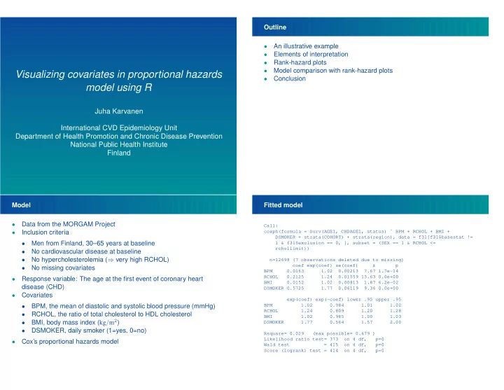
Fitted model

Call: coxph(formula = Surv(AGE1, CHDAGE1, status) ˜ BPM + RCHOL + BMI + DSMOKER + strata(COHORT) + strata(region), data = f31[f31$basestat != 1 & f31$exclusion == 0, ], subset = (SEX == 1 & RCHOL <= rchollimit)) n=12698 (7 observations deleted due to missing) coef exp(coef) se(coef) z p BPM 0.0163 1.02 0.00213 7.67 1.7e-14 RCHOL 0.2125 1.24 0.01559 13.63 0.0e+00 BMI 0.0152 1.02 0.00813 1.87 6.2e-02 DSMOKER 0.5725 1.77 0.06119 9.36 0.0e+00 exp(coef) exp(-coef) lower .95 upper .95 BPM 1.02 0.984 1.01 1.02 RCHOL 1.24 0.809 1.20 1.28 BMI 1.02 0.985 1.00 1.03 DSMOKER 1.77 0.564 1.57 2.00 Rsquare= 0.029 (max possible= 0.679 ) Likelihood ratio test= 373

• n 4 df,

p=0 Wald test = 415

• n 4 df,

p=0 Score (logrank) test = 414

• n 4 df,

p=0

Elements of interpretation

• Study design
• The type of model
• Definition of the covariate
• Estimated model parameter
• Unit of measurement
• Distribution of the covariate in the cohort (e.g. how common is

smoking?) Interpreting the results

• p-value oriented interpretation
• In the fitted model BPM, RCHOL and DSMOKER are statistically

significant at 5 % risk level.

• Covariates in ascending order by the p-values: RCHOL,

DSMOKER, BPM, BMI.

• The p-values will change if covariates are added or removed ⇐

covariates in the model are correlated.

• Other interesting questions
• What is the epidemiological relevance of these risk factors?
• Is smoking a more serious risk factor of CHD than overweight in

the population?

• How the model will change if we add, remove or transform

covariates?

• How to visualize the fitted model?

First visualization attempt Relative risk as a function of covariate values

80 100 120 140 160 180 0.5 1.0 2.0 5.0 10.0 BPM relative hazard

First attempt: BPM vs RCHOL

80 100 120 140 160 180 0.5 1.0 2.0 5.0 10.0 BPM relative hazard 2 4 6 8 10 12 14 0.5 1.0 2.0 5.0 10.0 RCHOL relative hazard

Information on the covariate distributions still not fully utilized.

Second attempt: ranks Relative risk as a function of ranks of covariate values

80 100 120 140 160 180 0.5 1.0 2.0 5.0 10.0 BPM relative hazard 0.0 0.2 0.4 0.6 0.8 1.0 0.5 1.0 2.0 5.0 10.0 cumulative covariate distribution relative hazard BPM (median=111.5 mmHg)

R implementation n<-length(x) x<-sort(x) relativehazard<-exp(beta*(x-median(x))) plot((1:n)/n,relativehazard,type="l",log="y") Rank-hazard plot Reference: medians

0.0 0.2 0.4 0.6 0.8 1.0 0.5 1.0 2.0 5.0 10.0 cumulative covariate distribution relative hazard BPM (median=111.5 mmHg) RCHOL (median=4.64 ) BMI (median=26.17 kg/m^2) DSMOKER

Rank-hazard plot Reference: normal upper limits

0.0 0.2 0.4 0.6 0.8 1.0 0.5 1.0 2.0 5.0 10.0 cumulative covariate distribution relative hazard BPM (reference=107.5 mmHg) RCHOL (reference= 5 ) BMI (reference= 25 kg/m^2) DSMOKER

Rank-hazard plot

0.0 0.2 0.4 0.6 0.8 1.0 0.5 1.0 2.0 5.0 10.0 cumulative covariate distribution relative hazard BPM (median=111.5 mmHg) RCHOL (median=4.64 ) BMI (median=26.17 kg/m^2) DSMOKER 0.0 0.2 0.4 0.6 0.8 1.0 0.5 1.0 2.0 5.0 10.0 cumulative covariate distribution relative hazard BPM (reference=107.5 mmHg) RCHOL (reference= 5 ) BMI (reference= 25 kg/m^2) DSMOKER

Model comparison Model with logarithms of covariates

0.0 0.2 0.4 0.6 0.8 1.0 0.5 1.0 2.0 5.0 10.0 cumulative covariate distribution relative hazard log(BPM) (median=4.714 ) log(RCHOL) (median=1.535 ) log(BMI) (median=3.265 ) DSMOKER

Model comparison

0.0 0.2 0.4 0.6 0.8 1.0 0.5 1.0 2.0 5.0 10.0 cumulative covariate distribution relative hazard BPM (median=111.5 mmHg) RCHOL (median=4.64 ) BMI (median=26.17 kg/m^2) DSMOKER 0.0 0.2 0.4 0.6 0.8 1.0 0.5 1.0 2.0 5.0 10.0 cumulative covariate distribution relative hazard log(BPM) (median=4.714 ) log(RCHOL) (median=1.535 ) log(BMI) (median=3.265 ) DSMOKER

Model comparison Model without blood pressure

0.0 0.2 0.4 0.6 0.8 1.0 0.5 1.0 2.0 5.0 10.0 cumulative covariate distribution relative hazard RCHOL (median= 4.64 ) BMI (median=26.17 kg/m^2) DSMOKER

Model comparison

0.0 0.2 0.4 0.6 0.8 1.0 0.5 1.0 2.0 5.0 10.0 cumulative covariate distribution relative hazard BPM (median=111.5 mmHg) RCHOL (median=4.64 ) BMI (median=26.17 kg/m^2) DSMOKER 0.0 0.2 0.4 0.6 0.8 1.0 0.5 1.0 2.0 5.0 10.0 cumulative covariate distribution relative hazard RCHOL (median= 4.64 ) BMI (median=26.17 kg/m^2) DSMOKER

Model comparison Adding history of diabetes

0.0 0.2 0.4 0.6 0.8 1.0 0.5 1.0 2.0 5.0 10.0 cumulative covariate distribution relative hazard BPM (median=111.5 mmHg) RCHOL (median= 4.64 ) BMI (median=26.17 kg/m^2) DSMOKER HISDIAB

Model comparison

0.0 0.2 0.4 0.6 0.8 1.0 0.5 1.0 2.0 5.0 10.0 cumulative covariate distribution relative hazard BPM (median=111.5 mmHg) RCHOL (median=4.64 ) BMI (median=26.17 kg/m^2) DSMOKER 0.0 0.2 0.4 0.6 0.8 1.0 0.5 1.0 2.0 5.0 10.0 cumulative covariate distribution relative hazard BPM (median=111.5 mmHg) RCHOL (median= 4.64 ) BMI (median=26.17 kg/m^2) DSMOKER HISDIAB

Conclusion

• Rank-hazard plots visualize several covariates in the same plot.
• Visualization may help interpreting the epidemiological relevance of

the covariates.

• Visualization is easy to implement in R.
• Future directions: How to visualize correlation between the covariates

in rank-hazard plots?