Recap: variance/covariance structure for linear mixed models - - PowerPoint PPT Presentation

Recap: variance/covariance structure for linear mixed models

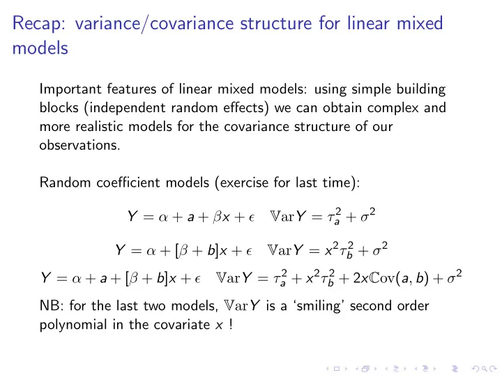
Important features of linear mixed models: using simple building blocks (independent random effects) we can obtain complex and more realistic models for the covariance structure of our

• bservations.

Random coefficient models (exercise for last time): Y = α + a + βx + ǫ VarY = τ 2

a + σ2

Y = α + [β + b]x + ǫ VarY = x2τ 2

b + σ2

Y = α + a + [β + b]x + ǫ VarY = τ 2

a + x2τ 2 b + 2xCov(a, b) + σ2

NB: for the last two models, VarY is a ‘smiling’ second order polynomial in the covariate x !

Variance is sum of covariances between random terms: VarY =Var(α + a + βx + bx + ǫ) = Cov(a, a) + Cov(a, bx) + Cov(bx, bx) + Cov(bx, a) + Cov(ǫ, ǫ) = Var(a) + Var(bx) + Varǫ + 2xCov(a, b) = τ 2

a + x2τ 2 b + σ2 + 2xρτaτb

NB: a and b are assumed to be independent of ǫ so e.g. Cov(a, ǫ) = 0 NB: ρ = Corr(a, b) = Cov(a, b) √ VaraVarb ⇒ Cov(a, b) = ρτaτb

Orthodont data

Distance (related to jaw size) between pituitary gland and the pterygomaxillary fissure (two distinct points on human skull) for children of age 8-14 Distance versus age:

8 9 10 11 12 13 14 20 25 30 age distance

Orthodont data

Distance (related to jaw size) between pituitary gland and the pterygomaxillary fissure (two distinct points on human skull) for children of age 8-14 Distance versus age:

8 9 10 11 12 13 14 20 25 30 age distance

Distance versus age grouped according to child

age distance

20 25 30 8 9 10 11 12 13 14

Different intercepts for different children !

Variance of empirical mean for one-way anova (exercise 7)

Covariances: Cov[Yij, Yi′j′] =      i = i′ VarUi i = i′, j = j′ VarUi + Varǫij i = i′, j = j′ (1) (km)2Var ¯ Y·· =

• i,j,i′,j′

Cov[Yij, Yi′j′] =

• i,j

VarYij +

• i,j=j′

Cov[Yij, Yi′j′] = km(σ2 + τ 2) + km(m − 1)τ 2 That is, Var ¯ Y·· = 1 (mk)2

• kmσ2 + kmτ 2 + km(m − 1)τ 2

= τ 2 k + σ2 km

Design of experiment (exercise 9)

From expression of Var ¯ Y·· obvious that we should take k=100 if km (total number of experiments) fixed at 100. Suppose budget is 5000 kr. 200 fee for each lab and 10 kr. for each experiment. Then 5000 = k200 + km10 ⇔ m = 5000 − k200 10k = 500 − 20k k Thus we shall minimize Var ¯ Y·· = 1 k + 3 k 500−20k

k

= 1 k + 3 500 − 20k This gives optimal k = 18.