Variance; Continuous Random Variables 18.05 Spring 2014 Jeremy Orloff - - PowerPoint PPT Presentation

variance continuous random variables 18 05 spring 2014
SMART_READER_LITE
LIVE PREVIEW

Variance; Continuous Random Variables 18.05 Spring 2014 Jeremy Orloff - - PowerPoint PPT Presentation

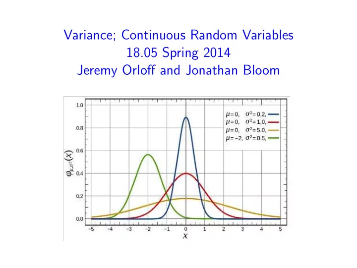
Variance; Continuous Random Variables 18.05 Spring 2014 Jeremy Orloff and Jonathan Bloom Variance and standard deviation X a discrete random variable with mean E ( X ) = . Meaning: spread of probability mass about the mean. Definition as


slide-1
SLIDE 1

Variance; Continuous Random Variables 18.05 Spring 2014 Jeremy Orloff and Jonathan Bloom

slide-2
SLIDE 2

Variance and standard deviation X a discrete random variable with mean E (X ) = µ. Meaning: spread of probability mass about the mean. Definition as expectation: Var(X ) = E ((X − µ)2). Computation as sum:

n

n Var(X ) = p(xi )(xi − µ)2 .

i=1

Standard deviation σ = Var(X ).

May 28, 2014 2 / 25

slide-3
SLIDE 3

Concept question

The graphs below give the pmf for 3 random variables. Order them by size of standard deviation from biggest to smallest.

x 1 2 3 4 5 (A) x 1 2 3 4 5 (B) x 1 2 3 4 5 (C)

  • 1. ABC
  • 2. ACB
  • 3. BAC
  • 4. BCA
  • 5. CAB
  • 6. CBA

Answer on next slide

May 28, 2014 3 / 25

slide-4
SLIDE 4

Solution

answer: 5. CAB All 3 variables have the same range from 1-5 and all of them are symmetric so their mean is right in the middle at 3. (C) has most of its weight at the extremes, so it has the biggest spread. (B) has the most weight in the middle so it has the smallest spread. From biggest to smallest standard deviation we have (C), (A), (B).

May 28, 2014 4 / 25

slide-5
SLIDE 5

Computation from tables

  • Example. Compute the variance and standard deviation
  • f X .

values x 1 2 3 4 5 pmf p(x) 1/10 2/10 4/10 2/10 1/10

Answer on next slide

May 28, 2014 5 / 25

slide-6
SLIDE 6

Computation from tables

From the table we compute the mean: 1 4 12 8 5 µ = + + + + = 3. 10 10 10 10 10 Then we add a line to the table for (X − µ)2 . values X 1 2 3 4 5 pmf p(x) 1/10 2/10 4/10 2/10 1/10 (X − µ)2 4 1 1 4 Using the table we compute variance E ((X − µ)2): 1 2 4 2 1 · 4 + · 1 + · 0 + · 1 + · 4 = 1.2 10 10 10 10 10 √ The standard deviation is then σ = 1.2.

May 28, 2014 6 / 25

slide-7
SLIDE 7

Concept question Which pmf has the bigger standard deviation?

  • 1. Y
  • 2. W

y p(y) 3

  • 3

1/2 pmf for Y w p(W) 10 20 30 40 50 .1 .2 .4 pmf for W

Board question: make probability tables for Y and W and compute their standard deviations.

Solution on next slide

May 28, 2014 7 / 25

slide-8
SLIDE 8

Solution

answer: We get the table for Y from the figure. After computing E(Y ) we add a line for (Y − µ)2 . Y

  • 3

3 p(y) .5 .5 (Y − µ)2 9 9 E (Y ) = .5(−3) + .5(3) = 0. E ((Y − µ)2) = .5(9) + .5(9) = 9 therefore Var(Y ) = 9 ⇒ σY = 3. W 10 20 30 40 50 p(w) .1 .2 .4 .2 .1 (W − µ)2 400 100 100 400 We compute E (W ) = 1 + 4 + 12 + 8 + 5 = 30 and add a line to the table for (W − µ)2 . Then Var(W ) = E ((W −µ)2) = .1(400)+.2(100)+.4(0)+.2(100)+.1(100) = 120 √ √ σW = 120 = 10 1.2. Note: Comparing Y and W , we see that scale matters for variance.

May 28, 2014 8 / 25

slide-9
SLIDE 9

Concept question True or false: If Var(X ) = 0 then X is constant.

  • 1. True
  • 2. False

answer: True. If X can take more than one value with positive probability, than Var(X ) will be a sum of positive terms. So X is constant if and only if Var(X ) = 0.

May 28, 2014 9 / 25

slide-10
SLIDE 10

Algebra with variances If a and b are constants then Var(aX + b) = a

2 Var(X ),

σaX +b = |a| σX . If X and Y are independent random variables then Var(X + Y ) = Var(X ) + Var(Y ).

May 28, 2014 10 / 25

slide-11
SLIDE 11

Board questions

  • 1. Prove: if X ∼ Bernoulli(p) then Var(X ) = p(1 − p).
  • 2. Prove: if X ∼ bin(n, p) then Var(X ) = n p(1 − p).
  • 3. Suppose X1, X2, . . . , Xn are independent and all have

the same standard deviation σ = 2. Let X be the average

  • f X1, . . . , Xn.

What is the standard deviation of X ?

Solution on next slide

May 28, 2014 11 / 25

slide-12
SLIDE 12

Solution

  • 1. For X ∼ Bernoulli(p) we use a table. (We know E (X ) = p.)

X 1 p(x) 1 − p p (X − µ)2 p2 (1 − p)2

2

Var(X ) = E ((X − µ)2) = (1 − p)p + p(1 − p)2 = p(1 − p)

  • 2. X ∼ bin(n, p) means X is the sum of n independent Bernoulli(p)

random variables X1, X2, . . . , Xn. For independent variables, the variances

  • add. Since Var(Xj ) = p(1 − p) we have

Var(X ) = Var(X1) + Var(X2) + . . . + Var(Xn) = np(p − 1). continued on next slide

May 28, 2014 12 / 25

slide-13
SLIDE 13

Solution continued

  • 3. Since the variables are independent, we have

Var(X1 + . . . + Xn) = 4n. X is the sum scaled by 1/n and the rule for scaling is Var(aX ) = a2Var(X ), so X1 + · · · + Xn 1 4 Var(X ) = Var( ) =

2 Var(X1 + . . . + Xn) = .

n n n 2 This implies σ = √ .

X

n Note: this says that the average of n independent measurements varies less than the individual measurements.

May 28, 2014 13 / 25

slide-14
SLIDE 14
  • Continuous random variables

Continuous range of values: [0, 1], [a, b], [0, ∞), (−∞, ∞). Probability density function (pdf) d f (x) ≥ 0; P(c ≤ x ≤ d) = f (x) dx.

c

Cumulative distribution function (cdf)

x

F (x) = P(X ≤ x) = f (t) dt.

−∞

May 28, 2014 14 / 25

slide-15
SLIDE 15

Visualization

x f(x) c d P(c ≤ X ≤ d)

pdf and probability

x f(x) x F(x) = P(X ≤ x)

pdf and cdf

May 28, 2014 15 / 25

slide-16
SLIDE 16

Properties of the cdf (Same as for discrete distributions) (Definition) F (x) = P(X ≤ x). 0 ≤ F (x) ≤ 1. non-decreasing. 0 to the left: lim F (x) = 0.

x→−∞

1 to the right: lim F (x) = 1.

x→∞

P(c < X ≤ d) = F (d) − F (c). F

'(x) = f (x).

May 28, 2014 16 / 25

slide-17
SLIDE 17

Board questions

2

  • 1. Suppose X has range [0, 2] and pdf f (x) = cx .

a) What is the value of c. b) Compute the cdf F (x). c) Compute P(1 ≤ X ≤ 2).

  • 2. Suppose Y has range [0, b] and cdf F (y) = y 2/9.

a) What is b? b) Find the pdf of Y .

Solution on next slide

May 28, 2014 17 / 25

slide-18
SLIDE 18
  • Solution
  • 1a. Total probability must be 1. So

2 2

8 3 f (x) dx = cx

2 dx = c

= 1 ⇒ c = . 3 8

  • 1b. The pdf f (x) is 0 outside of [0, 2] so for 0 ≤ x ≤ 2 we have

x 3

c x

3

F (x) = cu

2 du = x =

. 3 8 F (x) is 0 fo x < 0 and 1 for x > 2.

2

  • 1c. We could compute the probability as

f (x) dx, but rather than redo

1

the integral let’s use the cdf: 1 7 P(1 ≤ X ≤ 2) = F (2) − F (1) = 1 − = . 8 8 Continued on next slide

May 28, 2014 18 / 25

slide-19
SLIDE 19

Solution continued

  • 2a. Since the total probability is 1, we have

b2 F (b) = 1 ⇒ = 1 ⇒ 9 2y

  • 2b. f (y) = F

'(y) =

. 9 b = 3 .

May 28, 2014 19 / 25

slide-20
SLIDE 20

Concept questions Suppose X is a continuous random variable. a) What is P(a ≤ X ≤ a)? b) What is P(X = 0)? c) Does P(X = a) = 0 mean X never equals a?

answer: a) 0 b) 0 c) No. For a continuous distribution any single value has probability 0. Only a range of values has non-zero probability.

May 28, 2014 20 / 25

slide-21
SLIDE 21

Concept question

Which of the following are graphs of valid cumulative distribution functions? Add the numbers of the valid cdf’s and click that number.

answer: Test 2 and Test 3.

May 28, 2014 21 / 25

slide-22
SLIDE 22

Solution

Test 1 is not a cdf: it takes negative values, but probabilities are positive. Test 2 is a cdf: it increases from 0 to 1. Test 3 is a cdf: it increases from 0 to 1. Test 4 is not a cdf because it decreases. A cdf must be non-decreasing since it represents accumulated probability.

May 28, 2014 22 / 25

slide-23
SLIDE 23

Exponential Random Variables

Parameter: λ (called the rate parameter). Range: [0, ∞). Notation: exponential(λ) or exp(λ). Density: f (x) = λe−λx for 0 ≤ x. Models: Waiting times

x f(x) = λe−λx 2 4 6 8 10 12 14 16 λ

May 28, 2014 23 / 25

slide-24
SLIDE 24

Board question

I’ve noticed that taxis drive past 77 Mass. Ave. on the average of

  • nce every 10 minutes.

Suppose time spent waiting for a taxi is modeled by an exponential random variable X ∼ Exponential(1/10); f (x) = 1 10 e

−x/10

(a) Sketch the pdf of this distribution (b) Shade region which represents the probability of waiting between 3 and 7 minutes (c) Compute the probability of waiting between between 3 and 7 minutes for a taxi (d) Compute and sketch the cdf.

May 28, 2014 24 / 25

slide-25
SLIDE 25
  • Solution

Sketches for (a), (b), (d)

x P(3 < X < 7) 2 4 6 8 10 12 14 16 .1 x F(x) = 1 − e−x/10 2 4 6 8 10 12 14 16 1

(c)

7 7

1

−x/10 dx −x/10 −3/10 − e −7/10

(3 < X < 7) = e = −e = e = .244 10

3 3

May 28, 2014 25 / 25

slide-26
SLIDE 26