Outline Outline 2 Joint Cumulative Distribution Function (4.1, - - PowerPoint PPT Presentation

SLIDE 1

204312 PROBABILITY AND 204312 PROBABILITY AND RANDOM PROCESSES FOR COMPUTER ENGINEERS COMPUTER ENGINEERS

Lecture 6: Chapters 4.1-4.4 p

1st Semester, 2007 Monchai Sopitkamon, Ph.D.

Outline Outline

Joint Cumulative Distribution Function (4.1,

2

Joint Cumulative Distribution Function (4.1,

Y&G)

Joint Probabilit Mass F nction (4 2 Y&G) Joint Probability Mass Function (4.2, Y&G) Marginal PMF (4.3, Y&G) Joint Probability Density Function (4.4, Y&G)

Joint Cumulative Distribution Function I (4.1)

3

Experiments that produce two RVs, X and Y. E.g., signal X emitted by a radio transmitter, and the

g , g y , corresponding signal Y arriving at a receiver.

Observe Y and estimate X using prob. model fX Y (x, y) Observe Y and estimate X using prob. model fX, Y (x, y) E.g., strength of signal at a cell phone base station

receiver Y and the distance X of the phone from the receiver Y and the distance X of the phone from the base station.

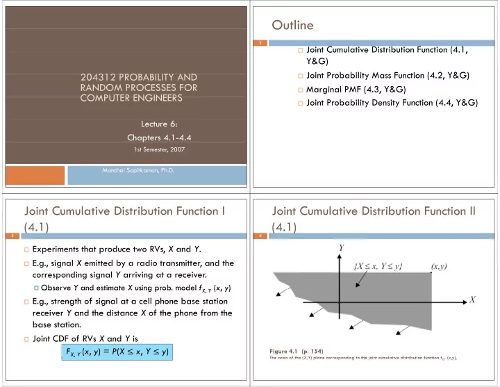
Joint CDF of RVs X and Y is

FX, Y (x, y) = P(X ≤ x, Y ≤ y)

Joint Cumulative Distribution Function II (4.1)

4

Figure 4.1 (p. 154)

The area of the (X Y) plane corresponding to the joint cumulative distribution function f (x y) The area of the (X,Y) plane corresponding to the joint cumulative distribution function fXY (x,y),

SLIDE 2

Joint Cumulative Distribution Function III (4.1)

5

For any pair of RVs X and Y

0 ≤ FX, Y (x, y) ≤ 1 X, Y FX (x) = P(X ≤ x, Y ≤ ∞) = FX, Y (x, ∞) F (y) = P(X ≤ ∞ Y ≤ y) = F

(∞ y)

FY (y) = P(X ≤ ∞, Y ≤ y) = FX, Y (∞, y) FX, Y (∞, ∞) = P(X ≤ ∞, Y ≤ ∞) =1 FX, Y (− ∞, y) = FX, Y (x, − ∞) = 0 If x ≤ x1 and y ≤ y1, then FX, Y (x, y) ≤ FX, Y (x1, y1) , ,

Joint Probability Mass Function I (4.2) Joint Probability Mass Function I (4.2)

6

f f

Joint prob. mass function of discrete RVs X and Y is:

) , ( ) , (

,

y Y x X P y x F

Y X

= = =

{X = x, Y = y} is an event in an experiment where

there is a set of observations that leads to both X = x and Y = y.

To find PX, Y (x, y), we sum the probabilities of all

X, Y

• utcomes of the experiment for which X = x and Y

= y.

Three ways to represent a joint PMF: a list, a matrix,

and a graph.

Joint Probability Mass Function II (4.2) Joint Probability Mass Function II (4.2)

7

Ex.4.1: Two-IC Test

Test two ICs one after the other. Possible outcomes are accepted (a) and rejected (r). Assume all Ics are acceptable with prob. 0.9 and outcomes of successive tests are independent. X counts the number of acceptable IC and Y counts the number of successful b f j tests before a reject.

Joint Probability Mass Function III (4.2) Joint Probability Mass Function III (4.2)

8

P(S) = 1, where S = sample space of the

experiment ∑ ∑

Or P

(x y) ≥ 0 for all pairs x y ∑ ∑

∈ ∈

=

X Y

S x S y Y X

y x P 1 ) , (

,

PX, Y (x, y) ≥ 0 for all pairs x, y For discrete RVs X and Y and any set B in the X, Y

l th b f th t {(X Y) B} i plane, the prob. of the event {(X, Y) ∈ B} is:

∑

=

Y X

y x P B P ) , ( ) (

∑

∈B y x Y X

y

) , ( ,

) , ( ) (

SLIDE 3

Joint Probability Mass Function IV (4.2) Joint Probability Mass Function IV (4.2)

9

Figure 4.2 (p. 157)

S b B f h (X Y) l P i (X Y) S k d b b ll Subsets B of the (X,Y) plane. Points (X,Y) ∈ SX,Y are marked by bullets.

Joint Probability Mass Function V (4.2) Joint Probability Mass Function V (4.2)

10

Ex.4.2: Find the prob. of the event B that X = Y

B ∩ SX, Y = {(0, 0), (1, 1), (2, 2)}

,

Therefore, P(B) = PX, Y (0, 0) + PX, Y (1, 1) + PX, Y (2, 2) = 0.01 + 0.09 + 0.81 0 0 0 09 = 0.91

Marginal PMF I (4.3) Marginal PMF I (4.3)

11

Consider just one of the RVs (e.g., Y) and ignore the

• ther one (e.g., X).

For discrete RVs X and Y with joint PMF PX, Y (x, y),

marginal PMF of X:

) ( ) (

∑

= y x P x F

marginal PMF of X: marginal PMF of Y:

, ) , ( ) (

,

∑

∈

=

y

S y Y X X

y x P x F ) ( ) (

∑

y x P y F

marginal PMF of Y:

. ) , ( ) (

,

∑

∈

=

X

S x Y X Y

y x P y F

Marginal PMF II (4.3) Marginal PMF II (4.3)

12

Ex.4.3: Find the marginal PMFs for the RVs X and Y. PX, Y (x, y) y = 0 y = 1 y = 2 x = 0 0.01 x = 1 0.09 0.09 x = 2 0.81

01 . ) , ( ) (

2 ,

= =∑

Y X X

y P P 18 . ) , 1 ( ) 1 (

2 ,

= =∑

Y X X

y P P

,

∑

= y ,

∑

= y

81 . ) , 2 ( ) 2 (

2 ,

= = ∑

= y Y X X

y P P 2 , 1 , ) ( ≠ = x x P

X = y

10 . ) , ( ) (

2 ,

= = ∑

= x Y X Y

x P P 09 . ) 1 , ( ) 1 (

2 ,

= = ∑

= x Y X Y

x P P 81 . ) 2 , ( ) 2 (

2 ,

= = ∑

= x Y X Y

x P P 2 , 1 , ) ( ≠ = y y P

Y

SLIDE 4

Marginal PMF III (4.3) Marginal PMF III (4.3)

13

Ex.4.3 (cont.): PX, Y (x, y) y = 0 y = 1 y = 2 PX (x) x = 0 0.01 0.01 x = 1 0.09 0.09 0.18 x = 2 0.81 0.81 PY (y) 0.10 0.09 0.81 ⎪ ⎪ ⎨ ⎧ = = 1 18 . 01 . ) ( x x x P ⎪ ⎪ ⎨ ⎧ = = 1 09 . 1 . ) ( y y y P ⎪ ⎪ ⎩ ⎨ = =

• therwise

2 81 . ) ( x x P

X

⎪ ⎪ ⎩ ⎨ = =

• therwise

2 81 . ) ( y y P

Y

Joint Probability Density Function I (4.4) Joint Probability Density Function I (4.4)

14

The joint PDF of the continuous RVs X and Y is a

function fX,Y (x, y) with the property

∫ ∫

∞ − ∞ −

=

x y Y X Y X

dvdu v u f y x F ) , ( ) , (

, ,

The joint PDF fX,Y (x, y) measures prob. per unit

area, whereas the PDF fX (x) measures prob. per

X

unit length.

fX Y (x, y) is a derivative of the CDF: fX,Y (x, y) is a derivative of the CDF:

y x F y x f

Y X Y X

∂ ∂ ∂ = ) , ( ) , (

, 2 ,

y x∂ ∂

,

Joint Probability Density Function II (4.4)

15

Properties of the joint PDF fX,Y (x, y): fX,Y (x, y) ≥ 0 for all (x, y) , . An event A corresponds to a region of the X, Y

1 ) , (

,

=

∫ ∫

∞ ∞ − ∞ ∞ −

y x f

Y X

An event A corresponds to a region of the X, Y

plane with the prob. of A being the double integral

• f f

(x y) over the region of the X Y plane

• f fX,Y (x, y) over the region of the X, Y plane

corresponding to A. Th b th t th ti RV (X Y) i A i

The prob. that the continuous RVs (X, Y) are in A is:

dy dx y x f A P

Y X

) , ( ) (

,

∫∫

=

A

Joint Probability Density Function III (4.4)

16

Ex.4.4: RVs X and Y have joint PDF

⎨ ⎧ ≤ ≤ ≤ ≤ = , 3 , 5 ) ( y x c y x f

Find the constant c and P(A) = P(2≤X<3, 1≤Y<3).

⎩ ⎨ =

• therwise.

) , (

,

y x f

Y X

From the fact that the integral of the joint PDF over the sample space is 1:

c dx dy c 15 1

5 3

= = ∫ ∫

Therefore, c = 1/15

c dx dy c 15 1 = = ∫ ∫

Therefore, c 1/15

15 / 2 15 1 ) (

3 2 3 1

= = ∫ ∫ du dv A P 15

SLIDE 5

Joint Probability Density Function IV (4.4)

17

Ex.4.5: Find the joint CDF FX,Y (x, y) when X and Y

have joint PDF

⎨ ⎧ ≤ ≤ ≤ = , 1 2 ) ( x y y x f ⎩ ⎨ =

• therwise.

) , (

,

y x f

Y X

fX,Y (x, y) = 2

FX,Y (x, y) = 0

Joint Probability Density Function IV (4.4)

18

Ex.4.5: Find the joint CDF FX,Y (x, y) when X and Y

have joint PDF

⎨ ⎧ ≤ ≤ ≤ = , 1 2 ) ( x y y x f ⎩ ⎨ =

• therwise.

) , (

,

y x f

Y X

FX,Y (x, y) = 1

Joint Probability Density Function IV (4.4)

19

Ex.4.5: Find the joint CDF FX,Y (x, y) when X and Y

have joint PDF

⎨ ⎧ ≤ ≤ ≤ = , 1 2 ) ( x y y x f ⎩ ⎨ =

• therwise.

) , (

,

y x f

Y X

2 ,

2 2 ) , ( y xy dv du y x F

y x v Y X

− = = ∫ ∫

, v

∫ ∫

Joint Probability Density Function IV (4.4)

20

Ex.4.5: Find the joint CDF FX,Y (x, y) when X and Y

have joint PDF

⎨ ⎧ ≤ ≤ ≤ = , 1 2 ) ( x y y x f ⎩ ⎨ =

• therwise.

) , (

,

y x f

Y X

2 ,

2 ) , ( x dv du y x F

x x v Y X

= = ∫ ∫

, v

∫ ∫

SLIDE 6

Joint Probability Density Function IV (4.4)

21

Ex.4.5: Find the joint CDF FX,Y (x, y) when X and Y

have joint PDF

⎨ ⎧ ≤ ≤ ≤ = , 1 2 ) ( x y y x f ⎩ ⎨ =

• therwise.

) , (

,

y x f

Y X

2 1 ,

2 2 ) , ( y y dv du y x F

y Y X

− = = ∫ ∫

,

∫ ∫

Joint Probability Density Function IV (4.4)

22

Ex.4.5: Find the joint CDF FX,Y (x, y) when X and Y

have joint PDF

⎨ ⎧ ≤ ≤ ≤ = , 1 2 ) ( x y y x f ⎩ ⎨ =

• therwise.

) , (

,

y x f

Y X

⎧ < < ) (

• r

a y x ⎪ ⎪ ⎪ ⎨ ⎧ ≤ ≤ < ≤ ≤ ≤ ≤ − < < = ) ( 1 , ) ( 1 2 ) (

• r

) , (

2 2

c x y x x b x y y xy a y x y x F

Y X

⎪ ⎪ ⎪ ⎩ ⎨ > > > ≤ ≤ − ) ( 1 , 1 1 ) ( 1 , 1 2 ) ( , ) , (

2 ,

e y x d x y y y y y

Y X

⎩ ) ( y

Joint Probability Density Function V (4.4)

23

If X and Y are RVs with joint PDF fX,Y (x, y),

) ( ) ( dy y x f x f

∫

∞

= ) ( ) ( dx y x f y f

∫

∞

=

E 4 7 Th j i t PDF f X

d Y i

, ) , ( ) (

,

dy y x f x f

Y X X

∫ ∞

−

= . ) , ( ) (

,

dx y x f y f

Y X Y

∫ ∞

−

=

Ex.4.7: The joint PDF of X and Y is

⎨ ⎧ ≤ ≤ ≤ ≤ − = , 1 , 1 1 4 / 5 ) , (

2

y x x y y x f

Y X

Find the marginal PDFs fX (x) and fY (y).

⎩ ⎨

• therwise.

) , (

,

y x f

Y X

Find the marginal PDFs fX (x) and fY (y).

HW4 (Due July 23, 2007) HW4 (Due July 23, 2007)

24

Problems 4.1.1 4.2.1 4.4.1 4 5 6 4.5.6 4.6.6