Random variables, expectation, and variance DSE 210 Random - - PDF document

Random variables, expectation, and variance

DSE 210

Random variables

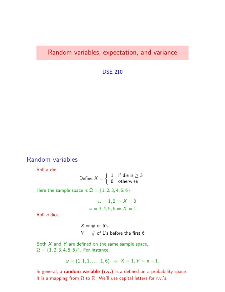
Roll a die. Define X = ⇢ 1 if die is ≥ 3

• therwise

Here the sample space is Ω = {1, 2, 3, 4, 5, 6}. ω = 1, 2 ⇒ X = 0 ω = 3, 4, 5, 6 ⇒ X = 1 Roll n dice. X = # of 6’s Y = # of 1’s before the first 6 Both X and Y are defined on the same sample space, Ω = {1, 2, 3, 4, 5, 6}n. For instance, ω = (1, 1, 1, . . . , 1, 6) ⇒ X = 1, Y = n − 1. In general, a random variable (r.v.) is a defined on a probability space. It is a mapping from Ω to R. We’ll use capital letters for r.v.’s.

The distribution of a random variable

Roll a die. Define X = 1 if die is ≥ 3, otherwise X = 0. X takes values in {0, 1} and has distribution: Pr(X = 0) = 1 3 and Pr(X = 1) = 2 3. Roll n dice. Define X = number of 6’s. X takes values in {0, 1, 2, . . . , n}. The distribution of X is: Pr(X = k) = #(sequences with k 6’s) · Pr(one such sequence) = ✓n k ◆ ✓1 6 ◆k ✓5 6 ◆n−k Throw a dart at a dartboard of radius 1. Let X be the distance to the center of the board. X takes values in [0, 1]. The distribution of X is: Pr(X ≤ x) = x2.

Expected value, or mean

The expected value of a random variable X is E(X) = X

x

x Pr(X = x). Roll a die. Let X be the number observed. E(X) = 1 · 1 6 + 2 · 1 6 + · · · + 6 · 1 6 = 1 + 2 + 3 + 4 + 5 + 6 6 = 3.5 (average) Biased coin. A coin has heads probability p. Let X be 1 if heads, 0 if tails. E(X) = 1 · p + 0 · (1 − p) = p. Toss a coin with bias p repeatedly, until it comes up heads. Let X be the number of tosses. E(X) = 1 p .

Pascal’s wager

Pascal: I think there is some chance (p > 0) that God exists. Therefore I should act as if he exists. Let X = my level of suffering.

I Suppose I behave as if God exists (that is, I behave myself).

Then X is some significant but finite amount, like 100 or 1000.

I Suppose I behave as if God doesn’t exists (I do whatever I want to).

If indeed God doesn’t exist: X = 0. But if God exists: X = ∞ (hell). Therefore, E(X) = 0 · (1 − p) + ∞ · p = ∞. The first option is much better!

Linearity of expectation

I If you double a set of numbers, how is the average affected?

It is also doubled.

I If you increase a set of numbers by 1, how much does the average

change? It also increases by 1.

I Rule: E(aX + b) = aE(X) + b for any random variable X and any

constants a, b.

I But here’s a more surprising (and very powerful) property:

E(X + Y ) = E(X) + E(Y ) for any two random variables X, Y .

I Likewise: E(X + Y + Z) = E(X) + E(Y ) + E(Z), etc.

Linearity: examples

Roll 2 dice and let Z denote the sum. What is E(Z)? Method 1 Distribution of Z: z 2 3 4 5 6 7 8 9 10 11 12 Pr(Z = z)

1 36 2 36 3 36 4 36 5 36 6 36 5 36 4 36 3 36 2 36 1 36

Now use formula for expected value: E(Z) = 2 · 1 36 + 3 · 2 36 + 4 · 3 36 + · · · = 7. Method 2 Let X1 be the first die and X2 the second die. Each of them is a single die and thus (as we saw earlier) has expected value 3.5. Since Z = X1 + X2, E(Z) = E(X1) + E(X2) = 3.5 + 3.5 = 7. Toss n coins of bias p, and let X be the number of heads. What is E(X)? Let the individual coins be X1, . . . , Xn. Each has value 0 or 1 and has expected value p. Since X = X1 + X2 + · · · + Xn, E(X) = E(X1) + · · · + E(Xn) = np. Roll a die n times, and let X be the number of 6’s. What is E(X)? Let X1 be 1 if the first roll is a 6, and 0 otherwise. E(X1) = 1 6. Likewise, define X2, X3, . . . , Xn. Since X = X1 + · · · + Xn, we have E(X) = E(X1) + · · · + E(Xn) = n 6.

Coupon collector, again

Each cereal box has one of k action figures. What is the expected number of boxes you need to buy in order to collect all the figures? Suppose you’ve already collected i − 1 of the figures. Let Xi be the time to collect the next one. Each box you buy will contain a new figure with probability (k − (i − 1))/k. Therefore, E(Xi) = k k − i + 1. Total number of boxes bought is X = X1 + X2 + · · · + Xk, so E(X) = E(X1) + E(X2) + · · · + E(Xk) = k k + k k − 1 + k k − 2 + · · · + k 1 = k ✓ 1 + 1 2 + · · · + 1 k ◆ ≈ k ln k.

Independent random variables

Random variables X, Y are independent if Pr(X = x, Y = y) = Pr(X = x)Pr(Y = y). Independent or not?

I Pick a card out of a standard deck. X = suit and Y = number.

Independent.

I Flip a fair coin n times. X = # heads and Y = last toss.

Not independent.

I X, Y take values {−1, 0, 1}, with the following probabilities:

Y

• 1

1

• 1

0.4 0.16 0.24 X 0.05 0.02 0.03 1 0.05 0.02 0.03 X Y

• 1

0.8 0.5 0.1 0.2 1 0.1 0.3 Independent.

Variance

If you had to summarize the entire distribution of a r.v. X by a single number, you would use the mean (or median). Call it µ. But these don’t capture the spread of X:

x Pr(x) x Pr(x) µ µ

What would be a good measure of spread? How about the average distance away from the mean: E(|X − µ|)? For convenience, take the square instead of the absolute value. Variance: var(X) = E(X − µ)2 = E(X 2) − µ2, where µ = E(X). The variance is always ≥ 0.

Variance: example

Recall: var(X) = E(X − µ)2 = E(X 2) − µ2, where µ = E(X). Toss a coin of bias p. Let X ∈ {0, 1} be the outcome. E(X) = p E(X 2) = p E(X − µ)2 = p2 · (1 − p) + (1 − p)2 · p = p(1 − p) E(X 2) − µ2 = p − p2 = p(1 − p) This variance is highest when p = 1/2 (fair coin). The standard deviation of X is p var(X). It is the average amount by which X differs from its mean.

Variance of a sum

var(X1 + · · · + Xk) = var(X1) + · · · + var(Xk) if the Xi are independent. Symmetric random walk. A drunken man sets out from a bar. At each time step, he either moves one step to the right or one step to the left, with equal probabilities. Roughly where is he after n steps? Let Xi ∈ {−1, 1} be his ith step. Then E(Xi) = ?0 and var(Xi) = ?1. His position after n steps is X = X1 + · · · + Xn. E(X) = 0 var(X) = n stddev(X) = √n He is likely to be pretty close to where he started!

Sampling

Useful variance rules:

I var(X1 + · · · + Xk) = var(X1) + · · · + var(Xk) if Xi’s independent. I var(aX + b) = a2var(X).

What fraction of San Diegans like sushi? Call it p. Pick n people at random and ask them. Each answers 1 (likes) or 0 (doesn’t like). Call these values X1, . . . , Xn. Your estimate is then: Y = X1 + · · · + Xn n . How accurate is this estimate? Each Xi has mean p and variance p(1 − p), so E(Y ) = E(X1) + · · · + E(Xn) n = p var(Y ) = var(X1) + · · · + var(Xn) n2 = p(1 − p) n stddev(Y ) = r p(1 − p) n ≤ 1 2√n

DSE 210: Probability and statistics Winter 2018

Worksheet 4 — Random variable, expectation, and variance

• 1. A die is thrown twice. Let X1 and X2 denote the outcomes, and define random variable X to be the

minimum of X1 and X2. Determine the distribution of X.

• 2. A fair die is rolled repeatedly until a six is seen. What is the expected number of rolls?
• 3. On any given day, the probability it will be sunny is 0.8, the probability you will have a nice dinner

is 0.25, and the probability that you will get to bed early is 0.5. Assume these three events are

• independent. What is the expected number of days before all three of them happen together?
• 4. An elevator operates in a building with 10 floors. One day, n people get into the elevator, and each of

them chooses to go to a floor selected uniformly at random from 1 to 10. (a) What is the probability that exactly one person gets out at the ith floor? Give your answer in terms of n. (b) What is the expected number of floors in which exactly one person gets out? Hint: let Xi be 1 if exactly one person gets out on floor i, and 0 otherwise. Then use linearity of expectation.

• 5. You throw m balls into n bins, each independently at random. Let X be the number of balls that end

up in bin 1. (a) Let Xi be the event that the ith ball falls in bin 1. Write X as a function of the Xi. (b) What is the expected value of X?

• 6. There is a dormitory with n beds for n students. One night the power goes out, and because it is dark,

each student gets into a bed chosen uniformly at random. What is the expected number of students who end up in their own bed?

• 7. In each of the following cases, say whether X and Y are independent.

(a) You randomly permute (1, 2, . . . , n). X is the number in the first position and Y is the number in the second position. (b) You randomly pick a sentence out of Hamlet. X is the first word in the sentence and Y is the second word. (c) You randomly pick a card from a pack of 52 cards. X is 1 if the card is a nine, and is 0 otherwise. Y is 1 if the card is a heart, and is 0 otherwise. (d) You randomly deal a ten-card hand from a pack of 52 cards. X is 1 if the hand contains a nine, and is 0 otherwise. Y is 1 if all cards in the hand are hearts, and is 0 otherwise.

• 8. A die has six sides that come up with different probabilities:

Pr(1) = Pr(2) = Pr(3) = Pr(4) = 1/8, Pr(5) = Pr(6) = 1/4. (a) You roll the die; let Z be the outcome. What is E(Z) and var(Z)? 4-1

DSE 210 Worksheet 4 — Random variable, expectation, and variance Winter 2018 (b) You roll the die 10 times, independently; let X be the sum of all the rolls. What is E(X) and var(X)? (c) You roll the die n times and take the average of all the rolls; call this A. What is E(A)? What is var(A)?

• 9. Let X1, X2, . . . , X100 be the outcomes of 100 independent rolls of a fair die.

(a) What are E(X1) and var(X1)? (b) Define the random variable X to be X1 X2. What are E(X) and var(X)? (c) Define the random variable Y to be X1 2X2 + X3. What is E(Y ) and var(Y )? (d) Define the random variable Z = X1 X2 + X3 X4 + · · · + X99 X100. What are E(Z) and var(Z)?

• 10. Suppose you throw m balls into n bins, where m n. For the following questions, give answers in

terms of m and n. (a) Let Xi be the number of balls that fall into bin i. What is Pr(Xi = 0)? (b) What is Pr(Xi = 1)? (c) What is E(Xi)? (d) What is var(Xi)?

• 11. Give an example of random variables X and Y such that var(X + Y ) 6= var(X) + var(Y ).
• 12. Suppose a fair coin is tossed repeatedly until the same outcome occurs twice in a row (that is, two

heads in a row or two tails in a row). What is the expected number of tosses?

• 13. In a sequence of coin tosses, a run is a series of consecutive heads or consecutive tails. For instance,

the longest run in HTHHHTTHHTHH consists of three heads. We are interested in the following question: when a fair coin is tossed n times, how long a run is the resulting sequence likely to contain? To study this, pick any k between 1 and n, and let Rk denote the number of runs of length exactly k (for instance, a run of length k +1 doesn’t count). In order to figure out E(Rk), we define the following random variables: Xi = 1 if a run of length exactly k begins at position i, where i  n k + 1. (a) What are E(X1) and E(Xn−k+1)? (b) What is E(Xi) for 1 < i < n k + 1? (c) What is E(Rk)? (d) What is, roughly, the largest k for which E(Rk) 1? 4-2

Modeling data with probability distributions

DSE 210

Distributional modeling

A useful way to summarize a data set:

• Fit a probability distribution to it.
• Simple and compact, and captures the big picture while smoothing
• ut the wrinkles in the data.
• In subsequent application, use distribution as a proxy for the data.

Which distributions to use? There exist a few distributions of great universality which occur in a surprisingly large number of problems. The three principal distributions, with ramifications throughout probability theory, are the binomial distribution, the normal distribution, and the Poisson distribution. – William Feller. Well, this is true in one dimension. For higher-dimensional data, we’ll use combinations of 1-d models: products and mixtures.

The binomial distribution

Binomial(n, p): the number of heads when n coins of bias (heads probability p) are tossed, independently. Suppose X has a binomial(n, p) distribution. EX = np var(X) = np(1 − p) Pr(X = k) = ✓n k ◆ pk(1 − p)n−k

Fitting a binomial distribution to data

Example: Upcoming election in a two-party country.

• You choose 1000 people at random and poll them.
• 600 say Democratic.

What is a good estimate for the fraction of votes the Democrats will get in the election? Clearly, 60%. More generally, you observe n tosses of a coin of unknown bias. k of them are heads. How to estimate the bias? p = k n

Maximum likelihood estimation

Let P be a class of probability distributions (Gaussians, Poissons, etc). Maximum likelihood principle: pick the distribution in P that makes the data maximally likely. That is, pick the p ∈ P that maximizes Pr(data|p). E.g. Suppose P is the class of binomials. We observe n coin tosses, and k of them are heads.

• Maximum likelihood : pick the bias p that maximizes

Pr(data|p) = pk(1 − p)nk.

• Maximizing this is the same as maximizing its log,

LL(p) = k ln p + (n − k) ln(1 − p).

• Set the derivative to zero.

LL0(p) = k p − n − k 1 − p = 0 ⇒ p = k n .

Maximum likelihood: a small caveat

You have two coins of unknown bias.

• You toss the first coin 10 times, and it comes out heads every time.

You estimate its bias as p1 = 1.0.

• You toss the second coin 10 times, and it comes out heads once.

You estimate its bias as p2 = 0.1. Now you are told that one of the coins was tossed 20 times and 19 of them came out heads. Which coin do you think it is?

• Likelihood under p1:

Pr(19 heads out of 20 tosses|bias = 1) = 0

• Likelihood under p2:

Pr(19 heads out of 20 tosses|bias = 0.1) = (0.1)19(0.9)1 The likelihood principle would choose the second coin. Is this right?

Laplace smoothing

A smoothed version of maximum-likelihood: when you toss a coin n times and observe k heads, estimate the bias as p = k + 1 n + 2. Laplace’s law of succession: What is the probability that the sun won’t rise tomorrow?

• Let p be the probability that the sun won’t rise on a randomly

chosen day. We want to estimate p.

• For the past 5000 years (= 1825000 days), the sun has risen every
• day. Using Laplace smoothing, estimate

p = 1 1825002.

The normal distribution

The normal (or Gaussian) N(µ, σ2) has mean µ, variance σ2, and density function p(x) = 1 (2πσ2)1/2 exp ✓ −(x − µ)2 2σ2 ◆ .

• 68.3% of the distribution lies within one standard deviation of the

mean, i.e. in the range µ ± σ

• 95.5% lies within µ ± 2σ
• 99.7% lies within µ ± 3σ

Maximum likelihood estimation of the normal

Suppose you see n data points x1, . . . , xn ∈ R, and you want to fit a Gaussian N(µ, σ2) to them. How to choose µ, σ?

• Maximum likelihood: pick µ, σ to maximize

Pr(data|µ, σ2) =

n

Y

i=1

✓ 1 (2πσ2)1/2 exp ✓ −(xi − µ)2 2σ2 ◆◆

• Work with the log, since it makes things easier:

LL(µ, σ2) = n 2 ln 1 2πσ2 −

n

X

i=1

(xi − µ)2 2σ2 .

• Setting the derivatives to zero, we get

µ = 1 n

n

X

i=1

xi σ2 = 1 n

n

X

i=1

(xi − µ)2 These are simply the empirical mean and variance.

Normal approximation to the binomial

= ⇒ When a coin of bias p is tossed n times, let X be the number of heads.

• We know X has mean np and variance np(1 − p).
• As n grows, the distribution of X looks increasingly like a Gaussian

with this mean and variance.

Application to sampling

We want to find out what fraction p of San Diegans know how to surf. So we poll n random people, and find that k of them surf. Our estimate: b p = k n . Normal approximation:

• k has a binomial(n, p) distribution.
• This is close to a Gaussian with mean np and variance np(1 − p).
• Therefore the distribution of b

p = k/n is close to a Gaussian with mean = p variance = p(1 − p) n ≤ 1 4n Confidence intervals:

• With 95% confidence, our estimate is accurate within ±1/√n.
• With 99% confidence, our estimate is accurate within ±3/2√n.

The multinomial distribution

A k-sided die:

• A fair coin has two possible outcomes, each equally likely.
• A fair die has six possible outcomes, each equally likely.
• Imagine a k-faced die, with probabilities p1, . . . , pk.

Toss such a die n times, and count the number of times each of the k faces occurs: Xj = # of times face j occurs The distribution of X = (X1, . . . , Xk) is called the multinomial.

• Parameters: p1, . . . , pk ≥ 0, with p1 + · · · + pk = 1.
• EX = (np1, np2, . . . , npk).
• Pr(n1, . . . , nk) =
• n

n1,n2,...,nk

• pn1

1 pn2 2 · · · pnk k , where

✓ n n1, n2, . . . , nk ◆ = n! n1!n2! · · · nk! is the number of ways to place balls numbered {1, . . . , n} into bins numbered {1, . . . , k}.

Example: text documents

Bag-of-words: vectorial representation of text documents.

It was the best of times, it was the

worst of times, it was the age of wisdom, it was the age of foolishness, it was the epoch of belief, it was the epoch of incredulity, it was the season of Light, it was the season of Darkness, it was the spring of hope, it was the winter of despair, we had everything before us, we had nothing before us, we were all going direct to Heaven, we were all going direct the

• ther way – in short, the period was

so far like the present period, that some of its noisiest authorities insisted on its being received, for good or for evil, in the superlative degree of comparison only.

despair evil happiness foolishness 1 1 2

• Fix V = some vocabulary.
• Treat the words in a document as independent draws from a

multinomial distribution over V : p = (p1, . . . , p|V |), such that pi ≥ 0 and X

i

pi = 1

The Poisson distribution

A distribution over the non-negative integers {0, 1, 2, . . .} The Poisson has parameter λ > 0, with Pr(X = k) = e−λ λk k!

• Mean: EX = λ
• Variance: E(X − λ)2 = λ
• Maximum likelihood fit: set λ to the empirical mean

How the Poisson arises

Count the number of events (collisions, phone calls, etc) that occur in a certain interval of time. Call this number X, and say it has expected value λ. Now suppose we divide the interval into small pieces of equal length. If the probability of an event occurring in a small interval is:

• independent of what happens in other small intervals, and
• the same across small intervals,

then X ∼ Poisson(λ).

Poisson: examples

Rutherford’s experiments with radioactive disintegration (1920)

radioactive substance counter

• N = 2608 intervals of 7.5 seconds
• Nk = # intervals with k particles
• Mean: 3.87 particles per interval

k 1 2 3 4 5 6 7 8 ≥ 9 Nk 57 203 383 525 532 408 273 139 45 43 P(3.87) 54.4 211 407 526 508 394 254 140 67.9 46.3

Flying bomb hits on London in WWII

• Area divided into 576 regions, each 0.25 km2
• Nk = # regions with k hits
• Mean: 0.93 hits per region

k 1 2 3 4 ≥ 5 Nk 229 211 93 35 7 1 P(0.93) 226.8 211.4 98.54 30.62 7.14 1.57

Multivariate distributions

Almost all distributions we’ve considered are for one-dimensional data.

• Binomial, Poisson: integer
• Gaussian: real

What to do with the usual situation of data in higher dimensions?

1 Model each coordinate separately and treat them as independent.

For x = (x1, . . . , xp), fit separate models Pri to each xi, and assume Pr(x1, . . . , xp) = Pr1(x1)Pr2(x2) · · · Prp(xp). This assumption is almost always completely inaccurate, and sometimes causes problems.

2 Multivariate Gaussian.

Allows modeling of correlations between coordinates.

3 More general graphical models.

Arbitrary dependencies between coordinates.

Classification with generative models 1

DSE 210

Machine learning versus Algorithms

In both fields, the goal is to develop procedures that exhibit a desired input-output behavior.

• Algorithms: the input-output mapping can be precisely defined.

Input: Graph G. Output: MST of G.

• Machine learning: the mapping cannot easily be made precise.

Input: Picture of an animal. Output: Name of the animal. Instead, we simply provide examples of (input,output) pairs and ask the machine to learn a suitable mapping itself.

Inputs and outputs

Basic terminology:

• The input space, X.

E.g. 32 × 32 RGB images of animals.

• The output space, Y.

E.g. Names of 100 animals. x: y: “bear” After seeing a bunch of examples (x, y), pick a mapping f : X → Y that accurately replicates the input-output pattern of the examples. Learning problems are often categorized according to the type of output space: (1) discrete, (2) continuous, (3) probability values, or (4) more general structures.

Discrete output space: classification

Binary classification:

• Spam detection

X = {email messages} Y = {spam, not spam}

• Credit card fraud detection

X = {descriptions of credit card transactions} Y = {fraudulent, legitimate} Multiclass classification:

• Animal recognition

X = {animal pictures} Y = {dog, cat, giraffe, . . .}

• News article classification

X = {news articles} Y = {politics, business, sports, . . .}

Continuous output space: regression

• Insurance company calculations

What is the expected age until which this person will live? Y = [0, 120]

• For the asthmatic

Predict tomorrow’s air quality (max over the whole day) Y = [0, ∞) (< 100: okay, > 200: dangerous) What are suitable predictor variables (X) in each case?

Conditional probability functions

Here Y = [0, 1] represents probabilities.

• Dating service

What is the probability these two people will go on a date if introduced to each other? If we modeled this as a classification problem, the binary answer would basically always be “no”. The goal is to find matches that are slightly less unlikely than others.

• Credit card transactions

What is the probability that this transaction is fraudulent? The probability is important, because – in combination with the amount of the transaction – it determines the overall risk and thus the right course of action.

Structured output spaces

The output space consists of structured objects, like sequences or trees. Dating service Input: description of a person Output: rank-ordered list of all possible matches Y = space of all permutations Example: x = Tom y = (Nancy, Mary, Chloe, . . .) Language processing Input: English sentence Output: parse tree showing grammatical structure Y = space of all trees Example: x = “John hit the ball” y =

A basic classifier: nearest neighbor

Given a labeled training set (x(1), y (1)), . . . , (x(n), y (n)). Example: the MNIST data set of handwritten digits. To classify a new instance x:

• Find its nearest neighbor amongst the x(i)
• Return y (i)

The data space

We need to choose a distance function. Each image is 28 ⇥ 28 grayscale. One

• ption:

Treat images as 784- dimensional vectors, and use Euclidean (`2) distance: kx x0k = v u u t

784

X

i=1

(xi x0

i )2.

Summary:

• Data space X = R784 with `2 distance
• Label space Y = {0, 1, . . . , 9}

Performance on MNIST

Training set of 60,000 points.

• What is the error rate on training points? Zero.

In general, training error is an overly optimistic predictor of future performance.

• A better gauge: separate test set of 10,000 points.

Test error = fraction of test points incorrectly classified.

• What test error would we expect for a random classifier? 90%.
• Test error of nearest neighbor: 3.09%.

Examples of errors: Query NN Properties of NN: (1) Can model arbitrarily complex functions (2) Unbounded in size

Classification with parametrized models

Classifiers with a fixed number of parameters can represent a limited set

• f functions. Learning a model is about picking a good approximation.

Typically the x’s are points in d-dimensional Euclidean space, Rd. Two ways to classify:

• Generative: model the individual classes.
• Discriminative: model the decision boundary between the classes.

Quick review of conditional probability

Formula for conditional probability: for any events A, B, Pr(A|B) = Pr(A ∩ B) Pr(B) . Applied twice, this yields Bayes’ rule: Pr(H|E) = Pr(E|H) Pr(E) Pr(H). Summation rule: Suppose events A1, . . . , Ak are disjoint events, one of which must occur. Then for any other event E, Pr(E) = Pr(E, A1) + Pr(E, A2) + · · · + Pr(E, Ak) = Pr(E|A1)Pr(A1) + Pr(E|A2)Pr(A2) + · · · + Pr(E|Ak)Pr(Ak)

Generative models

Generating a point (x, y) in two steps:

1 First choose y 2 Then choose x given y

Example: X = R Y = {1, 2, 3}

x Pr(x) P1(x) P2(x) P3(x) π1= 10% π2= 50% π3= 40%

The overall density is a mixture of the individual densities, Pr(x) = π1P1(x) + · · · + πkPk(x).

The Bayes-optimal prediction

x Pr(x) P1(x) P2(x) P3(x) π1= 10% π2= 50% π3= 40%

Labels Y = {1, 2, . . . , k}, density Pr(x) = π1P1(x) + · · · + πkPk(x). For any x ∈ X and any label j, Pr(y = j|x) = Pr(y = j)Pr(x|y = j) Pr(x) = πjPj(x) Pk

i=1 πiPi(x)

Bayes-optimal (minimum-error) prediction: h∗(x) = arg maxj πjPj(x).

A classification problem

You have a bottle of wine whose label is missing. Which winery is it from, 1, 2, or 3? Solve this problem using visual and chemical features of the wine.

The data set

Training set obtained from 130 bottles

• Winery 1: 43 bottles
• Winery 2: 51 bottles
• Winery 3: 36 bottles
• For each bottle, 13 features:

’Alcohol’, ’Malic acid’, ’Ash’, ’Alcalinity of ash’, ’Magnesium’, ’Total phenols’, ’Flavanoids’, ’Nonflavanoid phenols’, ’Proanthocyanins’, ’Color intensity’, ’Hue’, ’OD280/OD315 of diluted wines’, ’Proline’ Also, a separate test set of 48 labeled points.

Recall: the generative approach

x Pr(x) P1(x) P2(x) P3(x) π1= 10% π2= 50% π3= 40%

For any data point x ∈ X and any candidate label j, Pr(y = j|x) = Pr(y = j)Pr(x|y = j) Pr(x) = πjPj(x) Pr(x) Optimal prediction: the class j with largest πjPj(x).

Fitting a generative model

Training set of 130 bottles:

• Winery 1: 43 bottles, winery 2: 51 bottles, winery 3: 36 bottles
• For each bottle, 13 features: ’Alcohol’, ’Malic acid’, ’Ash’,

’Alcalinity of ash’,’Magnesium’, ’Total phenols’, ’Flavanoids’, ’Nonflavanoid phenols’, ’Proanthocyanins’, ’Color intensity’, ’Hue’, ’OD280/OD315 of diluted wines’, ’Proline’ Class weights: π1 = 43/130 = 0.33, π2 = 51/130 = 0.39, π3 = 36/130 = 0.28 Need distributions P1, P2, P3, one per class. Base these on a single feature: ’Alcohol’.

The univariate Gaussian

The Gaussian N(µ, σ2) has mean µ, variance σ2, and density function p(x) = 1 (2πσ2)1/2 exp ✓ −(x − µ)2 2σ2 ◆ .

The distribution for winery 1

Single feature: ’Alcohol’ Mean µ = 13.72, Standard deviation σ = 0.44 (variance 0.20)

All three wineries

• π1 = 0.33, P1 = N(13.7, 0.20)
• π2 = 0.39, P2 = N(12.3, 0.28)
• π3 = 0.28, P3 = N(13.2, 0.27)

To classify x: Pick the j with highest πjPj(x) Test error: 14/48 = 29%

DSE 210: Probability and statistics Winter 2018

Worksheet 5 — Classification with generative models 1

• 1. A man has two possible moods: happy and sad. The prior probabilities of these are:

π(happy) = 3 4, π(sad) = 1 4. His wife can usually judge his mood by how talkative he is. After much observation, she has noticed that:

• When he is happy,

Pr(talks a lot) = 2 3, Pr(talks a little) = 1 6, Pr(completely silent) = 1 6

• When he is sad,

Pr(talks a lot) = 1 6, Pr(talks a little) = 1 6, Pr(completely silent) = 2 3 (a) Tonight, the man is just talking a little. What is his most likely mood? (b) What is the probability of the prediction in part (a) being incorrect?

• 2. Suppose X = [−1, 1] and Y = {1, 2, 3}, and that the individual classes have weights

π1 = 1 3, π2 = 1 6, π3 = 1 2 and densities P1, P2, P3 as shown below.

• 1

1 P1(x) 7/8 1/8

• 1

1 P2(x) 1

5-1

DSE 210 Worksheet 5 — Classification with generative models 1 Winter 2018

• 1

1 P3(x) 1/2

What is the optimal classifier h∗? Specify it exactly, as a function from X to Y. 5-2