Unified bijective framework for planar maps Olivier Bernardi - - PowerPoint PPT Presentation

FPSAC, Paris 2013 Olivier Bernardi (Brandeis University)

Joint work with ´ Eric Fusy (CNRS/LIX)

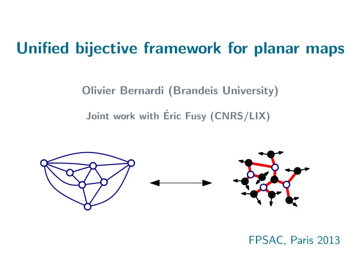
Unified bijective framework for planar maps

Maps Definition: A map is a gluing of polygons (pairing of the edges) forming a connected surface without boundary.

Maps

= =

Equivalent definition: A map is a cellular embedding of a connected graph in a surface, considered up to homeomorphism. Definition: A map is a gluing of polygons (pairing of the edges) forming a connected surface without boundary.

Planar maps. A planar map is a map on the sphere.

= =

Planar maps. A planar map is a map on the sphere. A planar triangulation.

Motivations

λ1 λ3 λ4λ5 λ6λ7 λ2 Random surfaces Permutations Random matrices

×

3 4 6 1 5 2 1 4 6 3 2 5 Algorithmic applications

Motivations

λ1 λ3 λ4λ5 λ6λ7 λ2 Random surfaces Permutations Random matrices

×

3 4 6 1 5 2 1 4 6 3 2 5 Algorithmic applications

Random surfaces

“There are methods and formulae in science, which serve as master-keys to many apparently different problems. The resources of such things have to be refilled from time to time. In my opinion at the present time we have to develop an art of handling sums over random surfaces. These sums replace the old-fashioned (and extremely useful) sums over random paths. ” A.M. Polyakov, Moscow, 1981

Random surfaces are important in physics (2D Quantum gravity)

Random surfaces Consider the random quadrangulation obtained by choosing uni- formly among all ways of gluing n = 1000 squares to form the sphere.

Random surfaces Consider the random quadrangulation obtained by choosing uni- formly among all ways of gluing n = 1000 squares to form the sphere. It is a random metric space: (Vn, dn). Hope to define a random surface by taking limit when

• number of squares → ∞,
• size of squares → 0.

Random surfaces Consider the random quadrangulation obtained by choosing uni- formly among all ways of gluing n = 1000 squares to form the sphere. It is a random metric space: (Vn, dn). Hope to define a random surface by taking limit when

• number of squares → ∞,
• size of squares → 0.

Theorem [Chassaing, Schaeffer 03] The distance between two random points of the random quadrangulations is Cn n1/4, where the random variable Cn converges in distribution toward a know law (ISE).

Random surfaces Let Mn = (Vn,

dn n1/4 ) be the random metric space corresponding to a

rescaled uniformly random quadrangulations with n squares.

Random surfaces Let Mn = (Vn,

dn n1/4 ) be the random metric space corresponding to a

rescaled uniformly random quadrangulations with n squares. Theorem.[Le Gall 2007 + Miermont/Le Gall 2012] The sequence (Mn) converges in distribution (in the Gromov Hausdorff topology) toward a random metric space, which

• is homeomorphic to the sphere
• has Hausdorff dimension 4.

(+ ”explicit” description of the space).

distribution

Related work. Bouttier, Di Francesco, Chassaing, Guitter, Le Gall, Marckert, Miermont, Mokkadem, Paulin, Schaeffer, Weill . . .

Key tool Bijection between quadrangulations and trees: [Cori, Vauquelin 81, Schaeffer 98]

Quadrangulation with n faces + marked vertex + marked edge Rooted plane tree with n edges +vertex labels changing by − 1, 0, 1 along edges and such that min=1. 2 2 1 1 1 3 3 2

Key tool Bijection between quadrangulations and trees: [Cori, Vauquelin 81, Schaeffer 98]

Quadrangulation with n faces + marked vertex + marked edge Rooted plane tree with n edges +vertex labels changing by − 1, 0, 1 along edges and such that min=1.

Vertex at distance d from marked vertex Vertex labeled d

2 2 1 1 1 3 3 2 2 1 1 3 3 2 1 2

A master bijection for planar maps

Counting formulas Example of counting formulas for rooted plane trees :

Binary trees (n nodes) k-ary trees (n nodes) 1 n + 1

• 2n

n

• 1

kn − n + 1

• kn

n

Counting formulas Example of counting formulas for rooted plane trees :

Binary trees (n nodes) k-ary trees (n nodes) 1 n + 1

• 2n

n

• 1

kn − n + 1

• kn

n

• Example of counting formulas for rooted planar maps [Tutte 60’s]:

Loopless triangulations Simple triangulations (2n triangles) (2n triangles) 2n (n + 1)(2n + 1)

• 3n

n

• 1

n(2n − 1)

• 4n − 2

n − 1

• General quadrangulations

Simple quadrangulations (2n squares) (2n squares) 2 · 3n (n + 1)(n + 2)

• 2n

n

• 2

n(n + 1)

• 3n

n − 1

A few bijections

• Triangulations (2n faces)
• Quadrangulations (n faces)
• Bipartite maps (ni faces of degree 2i)

Loopless: 2n (n + 1)(2n + 1) 3n n

• Simple:

1 n(2n − 1) 4n − 2 n − 1

• General:

2 · 3n (n + 1)(n + 2) 2n n

• Simple:

2 n(n + 1) 3n n − 1

• 2 · ( i ni)!

(2 + (i − 1)ni)!

• i

1 ni! 2i − 1 i ni [Poulalhon, Schaeffer 06 Fusy, Poulalhon, Schaeffer 08] [Schaeffer 97, Schaeffer 98] [Schaeffer 98, Fusy 07] [Schaeffer 97, Bouttier, Di Francesco, Guitter 04] [Poulalhon, Schaeffer 02, Bernardi 07]

Degree of the faces

Girth 1 2 3 4

1 2 3 4 5

6 7 8 A few bijections

Goal: Find a master bijection for planar maps which unifies all known bijections (of red type).

Goal:

• 1. Define a master bijection between a class of oriented maps

and a class of decorated trees.

• 2. Define canonical orientations for maps in any class defined by

degree and girth constraints. Find a master bijection for planar maps which unifies all known bijections (of red type). Strategy:

Goal: Find a master bijection for planar maps which unifies all known bijections (of red type). Alternative strategies:

• Bijection of the blue type [Albenque, Poulalhon 13+]
• Recursive decomposition by slices [Bouttier, Guitter 13+]

Oriented maps

external face external vertices

A plane map is a planar map with a distinguished “external face”.

Oriented maps Let O be the set of oriented plane maps such that:

• there is no counterclockwise directed cycle (minimal),
• internal vertices can be reached from external vertices (accessible),
• external vertices have indegree 1.

external face external vertices

A plane map is a planar map with a distinguished “external face”.

A mobile is a plane tree with vertices properly colored in black and white, together with buds (arrows) incident only to black vertices. Mobiles

Master bijection Mapping Φ for an oriented map in O:

• Return the external edges.
• Place a black vertex in each internal face.

Draw an edge/bud for each clockwise/counterclockwise edge.

• Erase the map.

Master bijection Theorem [B.,Fusy]: The mapping Φ is a bijection between the set O

• f oriented maps and the set of mobiles with more buds than edges.

Moreover, indegree of internal vertices ← → degree of white vertices degree of internal faces ← → degree of black vertices degree of external face ← → #buds - #edges

Master bijection: elements of proof Fact 1. Local operation in the faces produces a tree ← → Orientation is minimal and accessible.

Master bijection: elements of proof Fact 1. Local operation in the faces produces a tree ← → Orientation is minimal and accessible. Fact 2. The mobile captures all the info about the oriented map.

Canonical orientations

Goal:

Degree of faces

Girth 1 2 3 4

1 2 3 4 5

6 7 C= class of maps defined by girth constraints and degree constraints. We want to define a canonical orientation in O for each map in C C

How to define a canonical orientation? We consider a plane map M and want to define an orientation in O (orientations which are minimal + accessible + external indegree 1).

How to define a canonical orientation? We consider a plane map M and want to define an orientation in O (orientations which are minimal + accessible + external indegree 1). Fact 1: Let α be a function from the vertices of M to N. If there is an orientation of M with indegree α(v) for each vertex v, then there is unique minimal one. ⇒ Orientations in O can be defined by specifying the indegree α(v).

How to define a canonical orientation? We consider a plane map M and want to define an orientation in O (orientations which are minimal + accessible + external indegree 1). Fact 2: An orientation with indegree α(v) exists (and is accessible) if and only if

• v∈V

α(v) = |E|

• ∀U ⊂ V ,
• v∈U

α(v) ≥ |EU| (strict if there is an external vertex / ∈ U). Fact 1: Let α be a function from the vertices of M to N. If there is an orientation of M with indegree α(v) for each vertex v, then there is unique minimal one. ⇒ Orientations in O can be defined by specifying the indegree α(v).

How to define a canonical orientation? We consider a plane map M and want to define an orientation in O (orientations which are minimal + accessible + external indegree 1). Conclusion: For a map G, one can define an orientation in O by specifying an indegree function α such that:

• v∈V

α(v) = |E|,

• ∀ U ⊂ V ,
• v∈U

α(v) ≥ |EU| (strict if an external vertex / ∈ U),

• α(v) = 1 for every external vertex v.

How to define a canonical orientation? We consider a plane map M and want to define an orientation in O (orientations which are minimal + accessible + external indegree 1). Conclusion: For a map G, one can define an orientation in O by specifying an indegree function α such that:

• v∈V

α(v) = |E|,

• ∀ U ⊂ V ,
• v∈U

α(v) ≥ |EU| (strict if an external vertex / ∈ U),

• α(v) = 1 for every external vertex v.

Remark: Specifying indegrees is also convenient for master bijection: indegrees of internal vertices ← → degrees of white vertices.

Example: Simple triangulations

Degree of faces

Girth 1 2 3 4

1 2 3 4 5

6 7

Proof: The numbers v, e, f of vertices edges and faces satisfy:

• Incidence relation: 3f = 2e.
• Euler relation: v − e + f = 2.
• Example: Simple triangulations

Fact: A triangulation with n internal vertices has 3n internal edges.

Example: Simple triangulations Natural candidate for indegree function: α : v →

• 3 if v internal

1 if v external . Fact: A triangulation with n internal vertices has 3n internal edges. 1 1 1 3 3 3 3

Example: Simple triangulations New proof: Euler relation + the incidence relation ⇒ α satisfies:

v∈V α(v) = |E|,

• ∀ U ⊂ V ,

u∈U α(u) ≥ |EU| (strict if an external vertex /

∈ U),

• α(v) = 1 for every external vertex v.
• Thm.[Schnyder 89] A triangulation admits an orientation with indegree

function α if and only if it is simple.

Example: Simple triangulations Thm.[Schnyder 89] A triangulation admits an orientation with indegree function α if and only if it is simple.

• faces have degree 3
• internal vertices have indegree 3

⇒ The class of simple triangulations is identified with the class of

• riented maps in O such that

Example: Simple triangulations

• black vertices have degree 3
• white vertices have degree 3

Thm [recovering FuPoSc08]: The master bijection Φ induces a bijection between simple triangulations and mobiles such that Thm.[Schnyder 89] A triangulation admits an orientation with indegree function α if and only if it is simple.

• faces have degree 3
• internal vertices have indegree 3

⇒ The class of simple triangulations is identified with the class of

• riented maps in O such that

Example: Simple triangulations

• black vertices have degree 3
• white vertices have degree 3

Thm [recovering FuPoSc08]: The master bijection Φ induces a bijection between simple triangulations and mobiles such that Thm.[Schnyder 89] A triangulation admits an orientation with indegree function α if and only if it is simple.

• faces have degree 3
• internal vertices have indegree 3

⇒ The class of simple triangulations is identified with the class of

• riented maps in O such that

Corollary: The number of rooted simple triangulations with 2n faces is 1 n(2n − 1) 4n − 2 n − 1

• .

More classes of maps

Orientations for d-angulations of girth d Fact: A d-angulation with (d−2)n internal vertices has dn internal edges. Natural candidate for indegree function: α : v →

• d/(d − 2) if v internal

1 if v external . . .

d = 5

Orientations for d-angulations of girth d Idea: We can look for an orientation of (d−2)G with indegree function α : v →

• d if v internal

1 if v external . Fact: A d-angulation with (d−2)n internal vertices has dn internal edges. 5 5 5 5 5 5 Natural candidate for indegree function: α : v →

• d/(d − 2) if v internal

1 if v external . . .

d = 5

Orientations for d-angulations of girth d 2 1 2 1 2 1 2 1 Thm [B., Fusy]: Let G be a d-angulation. G has girth d ← → G admits a weighted orientation with

• weight d − 2 per edges.
• ingoing weight d per internal vertex,
• ingoing weight 1 per external vertex.

i≤0 j >0 i>0 j >0 i+j = d−2

Orientations for d-angulations of girth d Proof: Use the Euler relation + incidence relation as before.

• 2

1 2 1 2 1 2 1 Thm [B., Fusy]: Let G be a d-angulation. G has girth d ← → G admits a weighted orientation with

• weight d − 2 per edges.
• ingoing weight d per internal vertex,
• ingoing weight 1 per external vertex.

Moreover, G admits a unique such orientation in O in this case.

i≤0 j >0 i>0 j >0 i+j = d−2

3 3 3 3 3 3 0

Orientations for maps of girth d

Degree of faces

Girth 1 2 3 4

1 2 3 4 5

6 7

Orientations for maps of girth d Thm [B., Fusy]: Let G be a map. G has girth d ← → G admits a weighted bi-orientation with

• weight d − 2 per edges.
• ingoing weight d per internal vertex,
• ingoing weight 1 per external vertex,
• outgoing weight d − deg per faces.

1 2 2 1 1 2 1 2 2 1

• 1

4 5

• 2
• 1

4

• 1 4

3 3 3 3 3 3 i≤0 j >0 i>0 j >0 i≤0 j ≤0 i+j = d−2

Moreover, G admits a unique such orientation in O in this case.

Master bijection for weighted bi-orientation Theorem [B., Fusy] There is a bijection between weighted bi-oriented plane maps in O and weighted mobiles. Moreover, weight of internal edges ← → weight of edges ingoing weight of internal vertices ← → weight of white vertices degree of internal faces ← → degree of black vertices

• utgoing weight of internal faces ←

→ weight of black vertices.

1 2 2 2 2 1 2 1 1 1

• 1

4 5

• 2
• 14
• 1

4 30 3 3 0 3 3 3 1 2 2 1 1 2 1 2 21

• 1

4 5

• 2
• 1

4

• 14

3 3 3 3 3 3

Canonical orientations + Master bijection

• edges have weight d − 2,
• white vertices have weight d,
• black vertices have weight d − deg.

Thm [B., Fusy]: There is a bijection between maps of girth d and weighted mobiles such that

1 2 2 2 2 1 2 1 1 1

• 1

4 5

• 2
• 14
• 1

4 30 3 3 0 3 3 3 12 21 1 2 1 2 21

• 1

4 5

• 2
• 1

4

• 14

3 3 3 3 3 3

Moreover, faces of degree d ← → black vertices of degree d.

Counting Thm[B., Fusy]: d-angulations of girth d. The generating function Fd(x) =

• d-angulation
• f girth d

x#faces is given by Fd(x) = Wd−2 −

d−3

• i=0

WiWd−2−i, and F ′

d(x) = (1 + W0)d,

where W0, W1, . . . , Wd−2 are defined by:

• ∀j < d − 2,

Wj =

• r
• i1,...,ir>0

i1+···+ir=j+2

Wi1 · · · Wir,

• Wd−2 = x(1 + W0)d−1.

Counting Thm[B., Fusy]: d-angulations of girth d. The generating function Fd(x) =

• d-angulation
• f girth d

x#faces is given by Fd(x) = Wd−2 −

d−3

• i=0

WiWd−2−i, and F ′

d(x) = (1 + W0)d,

where W0, W1, . . . , Wd−2 are defined by:

• ∀j < d − 2,

Wj =

• r
• i1,...,ir>0

i1+···+ir=j+2

Wi1 · · · Wir,

• Wd−2 = x(1 + W0)d−1.

Example d=5: W0 = W 2

1 + W2

W1 = W 3

1 + 2W1W2 + W3

W2 = W 4

1 + 3W 2 1 W2 + 2W1W3 + W 2 2

W3 = x(1 + W0)4

Counting Thm[B., Fusy]: Maps of girth d (having outer degree d). The generating function Fd(xd, xd

+ 1, ..)=

• maps of

girth d

• i

x#faces of deg i

i

is given by Fd = Wd−2 −

d−3

• j=−2

WjWd−2−j where ∀j ∈ [−2..d−3], Wj =

• r
• i1,...,ir>0

i1+···+ir=j+2

Wi1 · · · Wir, and ∀j ∈ [d−2..d], Wj = [uj+1]

• i

xi (u + uW0 + W−1 + u−1)i−1.

Extends case d = 1 [Bouttier, Di Francesco, Guitter 02]

Counting Thm[B., Fusy]: Maps of girth d (having outer degree d). The generating function Fd(xd, xd

+ 1, ..)=

• maps of

girth d

• i

x#faces of deg i

i

is given by Fd = Wd−2 −

d−3

• j=−2

WjWd−2−j where ∀j ∈ [−2..d−3], Wj =

• r
• i1,...,ir>0

i1+···+ir=j+2

Wi1 · · · Wir, and ∀j ∈ [d−2..d], Wj = [uj+1]

• i

xi (u + uW0 + W−1 + u−1)i−1. Corollaries: If the set of admissible face degrees is finite, then

• Algebraic generating function.
• Asymptotic number of maps: ∼ c n−5/2 ρn.

Extends case d = 1 [Bouttier, Di Francesco, Guitter 02] Extends case d=1 [Bender, Canfield 94]

Additional results and questions

Bijections for planar maps Master bijection approach covers

• Classes of maps defined by girth constraint + degree constraints.

Degree of the faces

Girth 1 2 3 4

1 2 3 4 5

6

[FuPoSc08] [Sc98] [Sc97,BoDiGu02] [PoSc02]

7 8

Bijections for planar maps Master bijection approach covers

• Classes of maps defined by girth constraint + degree constraints.
• Case d = 0 [Schaeffer 98, Bouttier, Di Francesco, Guitter 04].

Degree of the faces

Girth 1 2 3 4

1 2 3 4 5

6

[FuPoSc08] [Sc98] [Sc97,BoDiGu02] [PoSc02]

7 8

[Sc98,BoDiGu04]

Bijections for planar maps Master bijection approach covers

• Classes of maps defined by girth constraint + degree constraints.
• Case d = 0 [Schaeffer 98, Bouttier, Di Francesco, Guitter 04].
• d-angulations with non-facial girth at least d, generalizing [Fusy,

Poulalhon, Schaeffer 08,Fusy 09].

Degree of the faces

Girth 1 2 3 4

1 2 3 4 5

6

[FuPoSc08] [Sc98] [Sc97,BoDiGu02] [PoSc02]

7 8

[Sc98,BoDiGu04]

Bijections for planar maps Master bijection approach covers

• Classes of maps defined by girth constraint + degree constraints.
• Case d = 0 [Schaeffer 98, Bouttier, Di Francesco, Guitter 04].
• d-angulations with non-facial girth at least d, generalizing [Fusy,

Poulalhon, Schaeffer 08,Fusy 09].

• Bipolar orientated maps[Fusy, Poulalhon, Schaeffer 09].

Degree of the faces

Girth 1 2 3 4

1 2 3 4 5

6

[FuPoSc08] [Sc98] [Sc97,BoDiGu02] [PoSc02]

7 8

[Sc98,BoDiGu04]

Bijections for planar hypermaps Master bijection approach extends to hypermaps.

Bijections for planar hypermaps Master bijection approach extends to hypermaps. The master bijection generalizes bijections by [Bousquet-M´ elou, Schaeffer 00] (Constellations), [Bousquet-M´ elou, Schaeffer 02] (Ising model), [Bouttier, Di Francesco, Guitter 04] (Distances). The master bijection generalizes bijections by [Bousquet-M´ elou, Schaeffer 00] (Constellations), [Bousquet-M´ elou, Schaeffer 02] (Ising model), [Bouttier, Di Francesco, Guitter 04] (Distances).

More fun with girth constraints? +2 +1 |C| ≥ d +

• f inside C

σ(f) We know how to control more general girth constraints. Question: Can we prove new probabilistic results on the cycle lengths in random maps?

Higher genus? A version of the master bijection exists for maps on orientable surfaces [B., Chapuy 10]. Question: Can we find canonical orientations (hence bijections)?

Thanks.

• 1. Algorithmic applications
• 1. Meshed surfaces.
• 2. Graph drawing.

• 2. Relation with permutations.

1 2 6 3 4 5

π = (1, 3, 6, 2)(4, 5) σ = (1, 5, 6, 3, 4)(2) Map with n labelled edges ← → pairs of permutation of {1, 2, . . . , n}

• 2. Relation with permutations.

1 2 6 3 4 5

π = (1, 3, 6, 2)(4, 5) σ = (1, 5, 6, 3, 4)(2) Map with n labelled edges ← → pairs of permutation of {1, 2, . . . , n} Cycles of π ← → blue vertices Cycles of σ ← → red vertices Cycles of πσ ← → faces