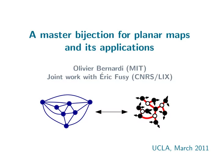
SLIDE 1
A master bijection for planar maps and its applications
UCLA, March 2011 Olivier Bernardi (MIT) Joint work with ´ Eric Fusy (CNRS/LIX)
SLIDE 2
A planar map is a connected planar graph embedded in the sphere considered up to continuous deformation. Planar maps. Definition
= =
SLIDE 3
- Algorithmic applications: efficient encoding of meshed surfaces.
- Probability and Physics: random lattices, random surfaces.
Appears courtesy to Wikipedia Appears courtesy to G. Chapuy
Planar maps. Motivations
- Representation Theory: factorization problems.
SLIDE 4
- Generating functions [Tutte 63]
Recursive description of maps recurrences.
- Matrix Integrals [’t Hooft 74]
Feynmann Diagram ≈ maps.
- Representation theory [Jackson 90]
Factorizations of permutations ≈ maps.
- Bijections [Cori-Vauquelin 91, Schaeffer 98]
Maps decorated trees. Planar maps. Methods
SLIDE 5
- Triangulations (2n faces)
- Quadrangulations (n faces)
- Bipartite maps (ni faces of degree 2i)
Planar maps. Counting results Common features: Algebraic generating function. Asymptotic ∼ κ n−5/2Rn.
Loopless: 2n (n + 1)(2n + 1) 3n n
1 n(2n − 1) 4n − 2 n − 1
2 · 3n (n + 1)(n + 2) 2n n
2 n(n + 1) 3n n − 1
(2 + (i − 1)ni)!
1 ni! 2i − 1 i ni
Planar maps. Counting results
SLIDE 6
- Triangulations (2n faces)
- Quadrangulations (n faces)
- Bipartite maps (ni faces of degree 2i)
[Sc97] [BoDiGu04] Loopless: 2n (n + 1)(2n + 1) 3n n
1 n(2n − 1) 4n − 2 n − 1
2 · 3n (n + 1)(n + 2) 2n n
2 n(n + 1) 3n n − 1
(2 + (i − 1)ni)!
1 ni! 2i − 1 i ni
Planar maps. Counting results
[ScPo02] [B.07] [Sc97] [Sc98] [PoSc06] [FuPoSc08] [Sc98] [Fu07] Bo: Bouttier Di: Di Francesco Fu: Fusy Gu: Guitter Po: Poulalhon Sc: Schaeffer Abbreviations:
SLIDE 7 Outline Benefits:
- Simplifies/unifies the proofs.
- Helps to find bijections for new classes of maps.
Describe a master bijection for planar maps which generalizes all the known bijections (of the red type).
SLIDE 8 Outline
- 1. Master bijection between a class of oriented maps and a class
- f bicolored decorated trees.
- 2. Specializations to classes of maps (via canonical orientations).
Degree of the faces
Girth 1 2 3 4
1 2 3 4 5
6
[FuPoSc08] [Sc98] [Sc98,BoDiGu04] [PoSc02]
7 8
SLIDE 9
Master bijection
(simplified version)
SLIDE 10
A plane orientation is a oriented map drawn in the plane. Plane orientations.
SLIDE 11 A plane orientation is a oriented map drawn in the plane. Plane orientations. We consider the set O of plane orientations which are:
- minimal: there is no counterclockwise directed cycle,
- accessible: any internal vertex can be reached from an external
vertex, and have external vertices of indegree 1.
SLIDE 12
A mobile is a plane tree with vertices properly colored in black and white, together with buds (half-edges) incident to black vertices. Mobiles The excess is the number of edges minus the number of buds.
SLIDE 13 Mapping Φ for a plane orientation O in O:
- Return the external face.
- Place a black vertex vf inside each internal face f.
Turning clockwise around f, draw an edge/bud from vf to the corners following forward/backward edges
- Erase the edges of O and its external vertices.
Master bijection
SLIDE 14 Master bijection Theorem [B.,Fusy]: The mapping Φ is a bijection between the set O
- f plane orientations and the set of mobiles with negative excess.
Moreover, indegree of internal vertices ← → degree of white vertices degree of internal faces ← → degree of black vertices degree of external face ← → - excess
SLIDE 15 Strategy for counting a class C of maps:
- Define a “canonical” orientation in O for each map in C.
This identifies C with a subset OC of O.
- Characterize (and count) the set of mobiles associated to OC via
the master bijection Φ. Using the master bijection to count classes of maps?
SLIDE 16
Using the master bijection to count classes of maps? How to define an orientation in the set O (orientations minimal, ac- cessible with external vertices of indegree 1)?
SLIDE 17
Using the master bijection to count classes of maps? Let G = (V, E) be a map and let α : V → N. How to define an orientation in the set O (orientations minimal, ac- cessible with external vertices of indegree 1)? Fact 1: If there exists an orientation of G with indegrees α(v), then there exists a unique minimal one. ⇒ Orientations O can be defined by specifying the indegrees.
SLIDE 18 Using the master bijection to count classes of maps? Let G = (V, E) be a map and let α : V → N. How to define an orientation in the set O (orientations minimal, ac- cessible with external vertices of indegree 1)? Fact 2: There exists an orientation with indegrees α(v) if and only if
v∈V α(v)
|EU| ≤
v∈U α(v).
Fact 1: If there exists an orientation of G with indegrees α(v), then there exists a unique minimal one. ⇒ Orientations O can be defined by specifying the indegrees.
SLIDE 19 Using the master bijection to count classes of maps? Let G = (V, E) be a map and let α : V → N. How to define an orientation in the set O (orientations minimal, ac- cessible with external vertices of indegree 1)? Fact 2: There exists an orientation with indegrees α(v) if and only if
v∈V α(v)
|EU| ≤
v∈U α(v).
Moreover, the orientation is accessible if and only if |EU| <
v∈U α(v)
whenever U does not contain all the external vertices. Fact 1: If there exists an orientation of G with indegrees α(v), then there exists a unique minimal one. ⇒ Orientations O can be defined by specifying the indegrees.
SLIDE 20 Using the master bijection to count classes of maps? Conclusion: For a map G = (V, E), one can define an orientation in O by specifying a function α : V → N such that:
- α(v) = 1 for every external vertex v,
- |E| =
v∈V α(v),
v∈U α(v)
with strict inequality if U does not contain all external vertices. (*)
SLIDE 21 Using the master bijection to count classes of maps? Conclusion: For a map G = (V, E), one can define an orientation in O by specifying a function α : V → N such that:
- α(v) = 1 for every external vertex v,
- |E| =
v∈V α(v),
v∈U α(v)
with strict inequality if U does not contain all external vertices. (*) Remark: Specifying an orientation in O by the indegrees of internal vertices is also convenient in view of applying the master bijection Φ: indegrees of internal vertices ← → degrees of white vertices.
SLIDE 22 Example of specialization: simple triangulations
Degree of faces
Girth 1 2 3 4
1 2 3 4 5
6 7
SLIDE 23 Proof: The numbers v, e, f of vertices edges and faces satisfy:
- Incidence relation: 3f = 2e.
- Euler relation: v − e + f = 2.
- Triangulations
Fact: A triangulation with n internal vertices has 3n internal edges.
SLIDE 24 Triangulations Natural candidate for indegree function: α : v →
1 if v external . Fact: A triangulation with n internal vertices has 3n internal edges. 1 1 1 3 3 3 3
SLIDE 25 Triangulations New (easier) proof: Use the Euler relation + the incidence relation to show that α satisfies condition (*).
- Thm [Schnyder 89]: A triangulation admits an orientation with in-
degree function α if and only if it is simple.
SLIDE 26 Triangulations ⇒ The class T of simple triangulations is indentified with the class of plane orientation OT ⊂ O with faces of degree 3, and internal vertices
Thm [recovering FuPoSc08]: By specializing the master bijection Φ to OT one obtains a bijection between simple triangulations and mobiles such that • black vertices have degree 3
- white vertices have degree 3
- the excess is −3 (redundant).
Thm [Schnyder 89]: A triangulation admits an orientation with in- degree function α if and only if it is simple.
SLIDE 27 Triangulations Counting: The generating function of mobiles with vertices of degree 3 rooted on a white corner is T(x) = U(x)3, where U(x) = 1 + xU(x)4. Consequently, the number of (rooted) simple triangulations with 2n faces is 1 n(2n − 1) 4n − 2 n − 1
SLIDE 28 More specializations: d-angulations of girth d.
Degree of faces
Girth 1 2 3 4
1 2 3 4 5
6 7
SLIDE 29 d-angulations of girth d Fact: A d-angulation with (d−2)n internal vertices has dn internal edges.
d = 5
SLIDE 30 d-angulations of girth d Fact: A d-angulation with (d−2)n internal vertices has dn internal edges. Natural candidate for indegree function: α : v →
1 if v external . . .
d = 5
SLIDE 31 d-angulations of girth d Idea: We can look for an orientation of (d−2)G with indegree function α : v →
1 if v external . Fact: A d-angulation with (d−2)n internal vertices has dn internal edges. 5 5 5 5 5 5
d = 5
SLIDE 32 d-angulations of girth d Proof: Use the Euler relation + incidence relation to show that α satisfies condition (*).
- Thm [B., Fusy]: Let G be a d-angulation. Then (d−2)G admits an
- rientation with indegree function α if and only if G has girth d.
2 1 2 1 2 1 2 1
d = 5
SLIDE 33 There are now white-white edges in the mobile, with two positive weights summing to d − 2. Master bijection for fractional orientations
2 1 2 1 1 2 21 2 1 2 1 1 2 21 2 1 2 1 1 2 21
SLIDE 34 Master bijection for fractional orientations Theorem [B.,Fusy]: Φ is a bijection between the set Ok of plane k- fractional orientations and the set of mobiles (with white-white edges having weights summing to k) with negative excess. Moreover, degree of internal faces ← → degree of black faces indegree of internal vertices ← → indegree of white vertices degree of external face ← → - excess
2 1 2 1 1 2 21 2 1 2 1 1 2 21 2 1 2 1 1 2 21
SLIDE 35 d-angulations of girth d ⇒ The class Td of d-angulations of girth d can be indentified with the class of fractional orientations Ωd ⊂ Od
− 2 with faces of degree d, and
internal vertices of indegree d.
2 1 2 1 2 1 2 1 2 1 1 2 21 21
Thm [B., Fusy]: Let G be a d-angulation. Then (d−2)G admits an
- rientation with indegree function α if and only if G has girth d.
SLIDE 36 d-angulations of girth d
- black vertices have degree d
- white vertices have indegree d
- the excess is −d (redundant).
2 1 2 1 2 1 2 1 2 1 1 2 21 21
Thm [B., Fusy]: By specializing the master bijection one obtains a bijection between d-angulations of girth d and mobiles (with white-white edges having weights summing to d − 2) such that Thm [B., Fusy]: Let G be a d-angulation. Then (d−2)G admits an
- rientation with indegree function α if and only if G has girth d.
SLIDE 37 d-angulations of girth d: counting Thm[B., Fusy]: Let W0, W1, . . . , Wd−2 be the power series in x defined by: Wd−2 = x(1 + W0)d−1 and ∀j < d − 2, Wj =
i1+···+ir=j+2
Wi1 · · · Wir. The generating function Fd of d-angulations of girth d satisfies Fd = Wd−2 −
d−3
WiWd−2−i, and F ′
d(x) = (1 + W0)d.
SLIDE 38 d-angulations of girth d: counting Thm[B., Fusy]: Let W0, W1, . . . , Wd−2 be the power series in x defined by: Wd−2 = x(1 + W0)d−1 and ∀j < d − 2, Wj =
i1+···+ir=j+2
Wi1 · · · Wir. The generating function Fd of d-angulations of girth d satisfies Fd = Wd−2 −
d−3
WiWd−2−i, and F ′
d(x) = (1 + W0)d.
Example d=5: W3 = x(1 + W0)4 W0 = W 2
1 + W2
W1 = W 3
1 + 2W1W2 + W3
W2 = W 4
1 + 3W 2 1 W2 + 2W1W3 + W 2 2
SLIDE 39 More specializations: Maps of girth d.
Degree of faces
Girth 1 2 3 4
1 2 3 4 5
6 7
SLIDE 40
Maps of girth d We consider maps of girth d with external face of degree d.
SLIDE 41 Maps of girth d Orientation: It is possible to characterize girth d by looking at
- rientations on (d−2)G + 2Q.
We consider maps of girth d with external face of degree d. Thm [B., Fusy]. Let G be a map with external face of degree d. The map G has girth d if and only if (d−2)G + 2Q admits an orientation such that inner vertices of G have indegree d and vertices of Q in faces
- f degree δ have indegree δ + d.
1 1 1 1 1 1
SLIDE 42 Maps of girth d Orientation: It is possible to characterize girth d by looking at
- rientations on (d−2)G + 2Q.
We consider maps of girth d with external face of degree d.
- Bijection. The orientation can be transfered to the map G and gives
a canonical orientation in O. One can characterize the mobiles obtained by the master bijection. (There are weights on the half-edges of the mobile. There are white- white and black-black edges. . . )
SLIDE 43 Maps of girth d Orientation: It is possible to characterize girth d by looking at
- rientations on (d−2)G + 2Q.
We consider maps of girth d with external face of degree d.
- Bijection. The orientation can be transfered to the map G and gives
a canonical orientation in O. One can characterize the mobiles obtained by the master bijection. Counting: The generating function Fd(xd, xd+1, . . .) of maps of girth d and outer degree d is Fd = Wd−2 −
d−3
WjWd−2−j. Where ∀j ∈ [−2..d−3], Wj =
i1+···+ir=j+2
Wi1 · · · Wir, and ∀j ∈ [d−2..d], Wj = [uj+1]
xi (u + uW0 + W−1 + u−1)i−1.
SLIDE 44 Closed formulas Prop [B.,Fusy]: The number of simple bipartite maps with ni faces
2((i + 1) ni − 3)! ( ini − 1)!
1 ni! 2i − 1 i + 1 ni 2 ( i ni)! ((i − 1)ni + 2)!
1 ni! 2i − 1 i ni This can be compared with the formula obtained by Schaeffer (97) for unconstrained bipartite maps:
SLIDE 45
Related results and extensions
SLIDE 46 Orientations for d-angulations as Schnyder decompositions Thm [B., Fusy] If G is a d-angulation of girth d, then one can partition the internal edges of (d − 2)G into d forests such that:
- each forest covers the internal vertices and d − 2 external vertices,
- the forests cross each other in a specific way.
SLIDE 47 Further extensions
- 1. The master bijection generalizes two other known bijections:
irreducible triangulations [FuPoSc08] and quadrangulations [Fu09].
Degree of the faces
Girth 1 2 3 4
1 2 3 4 5
6
[FuPoSc08] [Sc98] [Sc98,BoDiGu04] [PoSc02]
7 8
SLIDE 48 Further extensions
- 2. The master bijection can be extended to maps of higher genera.
[B., Chapuy 10].
- 1. The master bijection generalizes two other known bijections:
irreducible triangulations [FuPoSc08] and quadrangulations [Fu09].
SLIDE 49 Further extensions
- 2. The master bijection can be extended to maps of higher genera.
[B., Chapuy 10].
- 1. The master bijection generalizes two other known bijections:
irreducible triangulations [FuPoSc08] and quadrangulations [Fu09]. 3. The master bijection also generalizes some bijections for maps with matter.
SLIDE 50 Thanks.
On the ArXiv:
- A bijection for triangulations, quadrangulations, pentagulations, etc.
- Counting maps by girth and degree I. (number II in preparation)
Related:
- Schnyder decompositions for regular plane graphs and application to
drawing.
- A bijection for covered maps, or a shortcut between Harer-Zagier’s and
Jackson’s formulas, with Guillaume Chapuy (to appear in JCTA).
SLIDE 51
And now for something completely different. . . Schnyder woods and drawing algorithms
SLIDE 52 A Schnyder wood of a triangulation is a partition of the internal edges into 3 trees,
- each tree covers all the internal vertices and one external vertex,
- the trees cross in a specific manner around each internal vertex.
Schnyder woods for triangulations
SLIDE 53 Schnyder woods for triangulations Theorem [Schnyder 89,90].
- Any simple triangulation T admits a Schnyder wood.
- The Schnyder woods of T are in bijection with 3-orientations
(i.e. there exists a unique way of coloring each 3-orientation).
- It is possible to find a Schnyder wood of T in linear time.
- If T has n vertices, Schnyder woods can be used to compute a
planar straight-line drawing of T on the grid [2n] × [2n].
SLIDE 54
Prop: Any d-angulation of girth d admits a d/(d-2)-orientation (orientation of (d − 2)G such that the indegree of each vertex is d). Schnyder decompositions for d-angulations 5 5 5 5 5 5
SLIDE 55 Schnyder decompositions for d-angulations A Schnyder decomposition is a partition of (d − 2)E into d forests,
- each forest covers all the internal vertices and d − 2 external
vertices,
- the trees cross in a specific manner around each internal vertex.
SLIDE 56 Schnyder decompositions for d-angulations Theorem [B. Fusy].
- Any simple d-angulation T admits a Schnyder decomposition.
- The Schnyder woods of T are in bijection with its d/(d − 2)-
- rientations
(i.e. there exists a unique way of coloring each orientation).
- A Schnyder decomposition can be computed in polynomial time.
SLIDE 57 Dual of Schnyder decompositions (for d-regular graphs) A dual Schnyder decomposition is a collection of d spanning trees,
- each internal edge has two trees in opposite directions,
- the trees 1, 2, . . . , d arrive in this clockwise order at each vertex.
v∗
3 2 d d−1 1
SLIDE 58 Dual of Schnyder decompositions (for d-regular graphs) A dual Schnyder decomposition is a collection of d spanning trees,
- each internal edge has two trees in opposite directions,
- the trees 1, 2, . . . , d arrive in this clockwise order at each vertex.
Moreover, when d is even one can impose that for each edge e, the two trees using a of different parity. Trees 1 and 3 Trees 2 and 4
SLIDE 59 Application: drawing algorithm for 4-regular graphs Algorithm:
- For each vertex v, compute x(v)= number of faces on the left of v,
and y(v)=number of faces below v.
- Draw each vertex v at the point (x(v), y(v)) of the grid [n] × [n],
and draw each edge as a line segment. v x(v) faces
SLIDE 60
Application: drawing algorithm for 4-regular graphs Thm [B. Fusy]. The algorithm gives a straight-line planar drawing. The same vertex placement also gives an orthogonal planar drawing (with 1 bend per edge).