Part B: Mullin type bijections B.I Mullin bijection and - - PowerPoint PPT Presentation

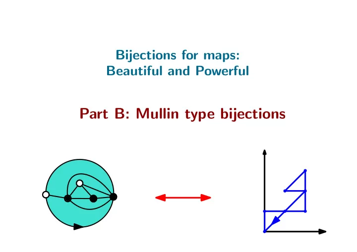
Bijections for maps: Beautiful and Powerful

Part B: Mullin type bijections

Mullin bijection and Sheffieldburger paradigm

B.I

Mullin’s bijection

• Def. A tree-decorated map is a map with a marked spanning tree.

Mullin’s bijection

• Def. A tree-decorated map is a map with a marked spanning tree.
• Remark. We have seen bijection between tree-decorated maps

with n edges and pairs of trees with n, n + 1 edges. Hence, # tree-decorated maps with n edges = CatnCatn+1 =

(2n)!(2n+2)! n!(n+1)!2(n+2)!.

Mullin’s bijection Thm.[Mullin 67, Lehman & Walsh 72] Tree-decorated maps with n edges are in bijection with lattice paths in N2 made of 2n steps →, ←, ↓, ↑, starting and ending at (0, 0).

Mullin’s bijection Def of Mullin bijection. Turn around the tree and write: → when following an edge of the tree for first time ← when following edge of tree for second time ↑ when crossing edge not in tree for first time ↓ when crossing edge not in tree for second time

Mullin’s bijection Def of Mullin bijection. Turn around the tree and write: → when following an edge of the tree for first time ← when following edge of tree for second time ↑ when crossing edge not in tree for first time ↓ when crossing edge not in tree for second time

Mullin’s bijection Def of Mullin bijection. Turn around the tree and write: → when following an edge of the tree for first time ← when following edge of tree for second time ↑ when crossing edge not in tree for first time ↓ when crossing edge not in tree for second time Easy to see it is bijection (...)

Mullin’s bijection Remark:: ↔ gives the contour code of the tree. gives the contour code of the dual tree. Hence the Mullin code is the shuffle of the two contour codes.

Mullin’s bijection Remark:: ↔ gives the contour code of the tree. gives the contour code of the dual tree. Hence the Mullin code is the shuffle of the two contour codes.

Mullin’s bijection Remark:: ↔ gives the contour code of the tree. gives the contour code of the dual tree. Hence the Mullin code is the shuffle of the two contour codes.

• Remark. This gives an easy way to count tree-decorated maps:

# tree decorated maps with n edges = n

k=0

2n

2k

• CatkCatn−k.

Other Mullin type bijections Percolation-decorated triangulations Schnyder-decorated triangulations

[Bernardi,Holden,Sun 19] [Bernardi 07] without [Bonichon 05] [Bernardi,Bonichon 09] [Li,Sun,Watson] [Kenyon, Miller, Sheffield, Wilson 15]

Bipolar-decorated triangulations

Other Mullin type bijections Question: Is there a master Mullin-type bijection for Gessel walks?

???

Other Mullin type bijections Question: Is there a master Mullin-type bijection for Gessel walks?

???

Question: Is there a master bijection for Mullin-type bijections?

Sheffield’s freshburgers Question: Mullin bijection is for tree-decorated maps. What about other subgraph-decorated maps?

Sheffield’s freshburgers Question: Mullin bijection is for tree-decorated maps. What about other subgraph-decorated maps? Idea: Associate every subgraph to a spanning tree (+ some marks), in order to obtain a bijection subgraph-decorated maps ← → marked tree-decorated maps.

Sheffield’s freshburgers

• Def. For lattice walk in N2 is called cone excursion if
• either it starts with ↑, ends with ↓ and remains at the right and

strictly above of the last step.

• or it starts with →, ends with ← and remains above and strictly

at the right of the last step.

Sheffield’s freshburgers

• Def. For a tree-decorated map, we call fresh an edge that corresponds

(via the Mullin encoding) to the last step of a cone excursion.

• Def. For lattice walk in N2 is called cone excursion if
• either it starts with ↑, ends with ↓ and remains at the right and

strictly above of the last step.

• or it starts with →, ends with ← and remains above and strictly

at the right of the last step. fresh

Sheffield’s freshburgers

• Def. For a tree-decorated map, we call fresh an edge that corresponds

(via the Mullin encoding) to the last step of a cone excursion.

• Def. For lattice walk in N2 is called cone excursion if
• either it starts with ↑, ends with ↓ and remains at the right and

strictly above of the last step.

• or it starts with →, ends with ← and remains above and strictly

at the right of the last step.

fresh fresh fresh fresh

Example.

Sheffield’s freshburgers

• Def. For a tree-decorated map, we call fresh an edge that corresponds

(via the Mullin encoding) to the last step of a cone excursion.

• Def. For lattice walk in N2 is called cone excursion if
• either it starts with ↑, ends with ↓ and remains at the right and

strictly above of the last step.

• or it starts with →, ends with ← and remains above and strictly

at the right of the last step.

Footnote 1: Why “fresh”? producing a cheeseburger eating a cheeseburger A step is fresh in the above sense if it corresponds to eating the freshest item currently available on the shelf. eating a hamburger producing a hamburger

Sheffield’s freshburgers

• Def. For a tree-decorated map, we call fresh an edge that corresponds

(via the Mullin encoding) to the last step of a cone excursion.

• Def. For lattice walk in N2 is called cone excursion if
• either it starts with ↑, ends with ↓ and remains at the right and

strictly above of the last step.

• or it starts with →, ends with ← and remains above and strictly

at the right of the last step.

Footnote 2: Given the spanning tree T, an edge e is “fresh” if it is the last edge to be visited within the cycle/cocycle it forms with T. This is similar to the notion of activity in the sense of the Tutte polynomial.

Sheffield’s freshburgers Lemma:[Bernardi 08/ Sheffield 12] 1. Every subgraph-decorated map is obtained in a unique way by adding/deleting some fresh edges to a tree-decorated map.

Sheffield’s freshburgers Lemma:[Bernardi 08/ Sheffield 12] 1. Every subgraph-decorated map is obtained in a unique way by adding/deleting some fresh edges to a tree-decorated map.

spanning trees and fresh edges (x) subgraphs obtained by adding/deleting edges

Example:

Sheffield’s freshburgers Lemma:[Bernardi 08/ Sheffield 12] 1. Every subgraph-decorated map is obtained in a unique way by adding/deleting some fresh edges to a tree-decorated map.

• 2. Moreover,

#connected components of subgraph = 1+ #fresh edges deleted. # cycles of subgraph (nullity) = # fresh edges added.

Sheffield’s freshburgers Lemma:[Bernardi 08/ Sheffield 12] 1. Every subgraph-decorated map is obtained in a unique way by adding/deleting some fresh edges to a tree-decorated map.

• 2. Moreover,

#connected components of subgraph = 1+ #fresh edges deleted. # cycles of subgraph (nullity) = # fresh edges added. Corollary:

• (M,S), n edges

subgraph-decorated map

xc(S)−1 yn(S) =

• W walk on N2, 2n steps

+ some marked fresh edges

xfresh← yfresh ↓.

Sheffield’s freshburgers Lemma:[Bernardi 08/ Sheffield 12] 1. Every subgraph-decorated map is obtained in a unique way by adding/deleting some fresh edges to a tree-decorated map.

• 2. Moreover,

#connected components of subgraph = 1+ #fresh edges deleted. # cycles of subgraph (nullity) = # fresh edges added.

Partition function of FK-cluster model on maps (⇐ ⇒ Potts model on maps) (⇐ ⇒ Tutte polynomial of maps)

Corollary:

Partition function of quarter-walks counted by size and #fresh steps

# connected components # fresh marked edges nullity

• (M,S), n edges

subgraph-decorated map

xc(S)−1 yn(S) =

• W walk on N2, 2n steps

+ some marked fresh edges

xfresh← yfresh ↓.

Sheffield’s freshburgers

• (M,S), n edges

subgraph-decotated map qc(S)−1+n(S) =

• W walk on N2, n steps

+ some marked fresh edges q#marked fresh. Critical FK-cluster model on maps (q determines the central charge)

Sheffield’s freshburgers

• (M,S), n edges

subgraph-decotated map qc(S)−1+n(S) =

• W walk on N2, n steps

+ some marked fresh edges q#marked fresh. Critical FK-cluster model on maps (q determines the central charge)

Rk: q ր ⇐ ⇒ fresh steps ր ⇐ ⇒ correlation of coordinates ր.

Sheffield’s freshburgers

• (M,S), n edges

subgraph-decotated map qc(S)−1+n(S) =

• W walk on N2, n steps

+ some marked fresh edges q#marked fresh. Critical FK-cluster model on maps (q determines the central charge)

Rk: q ր ⇐ ⇒ fresh steps ր ⇐ ⇒ correlation of coordinates ր.

α(q) Brownian excursion with correlated coordinates Brownian excursion in a cone

⇐ ⇒

Sheffield’s freshburgers

• (M,S), n edges

subgraph-decotated map qc(S)−1+n(S) =

• W walk on N2, n steps

+ some marked fresh edges q#marked fresh. Critical FK-cluster model on maps (q determines the central charge)

Theorem: [Sheffield 16] For q ∈ [0, 4] the scaling limit of fresh-weighted walks is a Brownian motion in a cone of angle α(q). Rk: q ր ⇐ ⇒ fresh steps ր ⇐ ⇒ correlation of coordinates ր.

α(q) Brownian excursion with correlated coordinates Brownian excursion in a cone

⇐ ⇒

Sheffield’s freshburgers

• (M,S), n edges

subgraph-decotated map qc(S)−1+n(S) =

• W walk on N2, n steps

+ some marked fresh edges q#marked fresh. Critical FK-cluster model on maps (q determines the central charge)

Theorem: [Sheffield 16] For q ∈ [0, 4] the scaling limit of fresh-weighted walks is a Brownian motion in a cone of angle α(q). Example: α(0) = π/2 for tree-decorated, α(1) = 2π/3 for percolation, α(2) = 3π/8 for Ising. Rk: q ր ⇐ ⇒ fresh steps ր ⇐ ⇒ correlation of coordinates ր.

α(q) Brownian excursion with correlated coordinates Brownian excursion in a cone

⇐ ⇒

Mating of trees [Duplantier, Miller, Sheffield] There is a parallel story in the context of Liouville quantum gravity:

Mating of trees [Duplantier, Miller, Sheffield] There is a parallel story in the context of Liouville quantum gravity: Theorem: [Duplantier, Miller, Sheffield 14] Grow a space-filling SLEκ(q) on LQGγ(q) and record length of sides. This process is equal to the “correlated” 2D-Brownian motion which is the limit of q-fresh-weighted walks. Moreover, the above is a σ-algebra preserving correspondence.

Mating of trees [Duplantier, Miller, Sheffield] There is a parallel story in the context of Liouville quantum gravity: Theorem: [Duplantier, Miller, Sheffield 14] Grow a space-filling SLEκ(q) on LQGγ(q) and record length of sides. This process is equal to the “correlated” 2D-Brownian motion which is the limit of q-fresh-weighted walks. Moreover, the above is a σ-algebra preserving correspondence. Gives hope of connecting (FK-weighted) maps to LQG and SLE via the walk encoding.

Percolated triangulations and a bijective path to LQG

B.II

Percolation on triangulation CLE on Liouville Quantum Gravity

Percolation on triangulation CLE on Liouville Quantum Gravity “Random curves on a random surface”

Percolation on triangulation CLE on Liouville Quantum Gravity Kreweras excursion 2D Brownian excursion

Percolation on triangulations

Percolation on a regular lattice Triangular lattice

Percolation on a regular lattice Site percolation: Color vertices black or white with probability 1/2.

Percolation on a regular lattice Questions:

• Crossing probabilities?

A n × B n box Site percolation: Color vertices black or white with probability 1/2.

Percolation on a regular lattice Questions:

• Crossing probabilities?
• Law of interfaces?

Site percolation: Color vertices black or white with probability 1/2.

• Crossing probabilities?

Percolation on a regular lattice Questions:

• Crossing probabilities?
• Law of interfaces?
• Mixing properties?

Site percolation: Color vertices black or white with probability 1/2.

• Crossing probabilities?

Triangulations (of the disk)

• Def. A triangulation of the disk is a decomposition into triangles.

Triangulations (of the disk) =

• Def. A triangulation of the disk is a decomposition into triangles

(considered up to deformation).

Triangulations (of the disk) (multiple edges allowed, loops forbidden)

• Def. A triangulation of the disk is a decomposition into triangles

(considered up to deformation).

Triangulations (of the disk)

• Def. A triangulation is rooted by marking an edge on the boundary.
• Def. A triangulation of the disk is a decomposition into triangles

(considered up to deformation).

Percolation on triangulations We can consider percolation on random triangulations of the disk. (k exterior vertices, n interior vertices; uniform probability)

Percolation on triangulations Same questions:

• Crossing probabilities?
• Law of interfaces?
• Mixing properties?

We can consider percolation on random triangulations of the disk. (k exterior vertices, n interior vertices; uniform probability)

Percolation on triangulations Same questions:

• Crossing probabilities?
• Law of interfaces?
• Mixing properties?

We can consider percolation on random triangulations of the disk. (k exterior vertices, n interior vertices; uniform probability) Goal 1: Answer these questions. (as n → ∞, k ∼ √n)

We can also consider infinite triangulations. Percolation on triangulations Same questions:

• Crossing probabilities?
• Law of interfaces?
• Mixing properties?

We can consider percolation on random triangulations of the disk. (k exterior vertices, n interior vertices; uniform probability) Uniform Infinite Planar Triangulation [Angel,Schramm 04] Goal 1: Answer these questions. (as n → ∞, k ∼ √n)

Regular lattices Vs random lattices Is it interesting to study statistical mechanics on random lattices? Vs regular lattice random lattice

Regular lattices Vs random lattices Is it interesting to study statistical mechanics on random lattices? Vs regular lattice random lattice Yes! New tools: random matrices, generating functions, bijections.

Regular lattices Vs random lattices Yes! The “critical exponents” on regular Vs random lattices are related by the KPZ formula [Knizhnik, Polyakov, Zamolodchikov]. Is it interesting to study statistical mechanics on random lattices? Vs regular lattice random lattice Yes! New tools: random matrices, generating functions, bijections.

Regular lattices Vs random lattices Yes! The “critical exponents” on regular Vs random lattices are related by the KPZ formula [Knizhnik, Polyakov, Zamolodchikov]. Yes! Critically weighted random lattices random surfaces. Is it interesting to study statistical mechanics on random lattices? Vs regular lattice random lattice Yes! New tools: random matrices, generating functions, bijections.

Liouville Quantum Gravity (LQG) and Schramm–Loewner Evolution (SLE)

What is . . . Liouville Quantum Gravity?

What is . . . Liouville Quantum Gravity? LQG is a random area measure µ on a C-domain which is related to the Gaussian free field.

(image by J. Miller)

What is . . . Liouville Quantum Gravity? 1D LQG Brownian motion 1 1D LQG 1

h µ = eγhdx

What is . . . Liouville Quantum Gravity?

Random function chosen with probability proportional to e −

n

• i=1

(h(i) − h(i − 1))2 2

Brownian motion 1D LQG 1D LQG

hn : [n] → R µ = eγhdx

1

h = lim hn

1 n

What is . . . Liouville Quantum Gravity?

hn : [n]2 → R µ = eγhdxdy h = lim hn Random function chosen with probability proportional to e −

• u∼v

(h(u) − h(v))2 2

Gaussian Free Field LQG

(a distribution) (area measure)

What is . . . Liouville Quantum Gravity?

hn : [n]2 → R µ = eγhdxdy h = lim hn γ ∈ [0, 2] controls how wild LQG measure is. Today: γ =

• 8/3.

“pure gravity”

What is... a SLE (Schramm–Loewner evolution)?

What is... a SLE (Schramm–Loewner evolution)? SLEκ is a random (non-crossing, parametrized) curve in a C-domain.

What is... a SLE (Schramm–Loewner evolution)? SLEκ were introduced to describe the scaling limit of curves from statistical mechanics. SLEκ is a random (non-crossing, parametrized) curve in a C-domain. The parameter κ determines how much the curve “wiggles”.

What is... a SLE (Schramm–Loewner evolution)? SLE are characterized by:

• Conformal invariance property
• Markov domain property

1 γ

What is... a SLE (Schramm–Loewner evolution)? SLE are characterized by:

• Conformal invariance property
• Markov domain property

1 1 φ conformal

γ(t)

What is... a SLE (Schramm–Loewner evolution)? SLE are characterized by:

• Conformal invariance property
• Markov domain property

1 1 ei√κW (t)

γ(t) Brownian

˜ φ conformal

What is... a SLE (Schramm–Loewner evolution)? Today: κ = 6 (percolation)

What is... a SLE (Schramm–Loewner evolution)? Today: κ = 6 (percolation) Theorem [Smirnov 01]: Convergence. SLE6

What is... a SLE (Schramm–Loewner evolution)? Today: κ = 6 (percolation) Theorem [Smirnov 01]: Convergence.

What is... a SLE (Schramm–Loewner evolution)? CLE6

Conformal Loop Ensemble

Today: κ = 6 (percolation) Theorem [Smirnov 01]: Convergence. Theorem [Camia, Newman 09]: Convergence.

The big conjecture

Riemann mapping

?

Nice embedding

The big conjecture under nice embedding

LQG√

8/3

LQG√

8/3 + CLE6

The big conjecture under nice embedding

bijection

[Bernardi 2007] σ-algebra preserving coupling [Bernardi, Holden, Sun 2019] LQG√

8/3 + CLE6

[Duplantier, Miller, Sheffield 2014] “mating of trees”

under nice embedding Strategy of proof

B.III

Bijection: Percolated triangulations ← → Kreweras walks

Kreweras walks Def. A Kreweras walk is a lattice walk on Z2 using the steps a = (1, 0), b = (0, 1) and c = (−1, −1). b a c

Thm [Bernardi 07/ Bernardi, Holden, Sun 18]: There is a bijection between:

• K = set of Kreweras walks starting and ending at (0, 0)

and staying in N2.

• T = set of percolated triangulations of the disk

with 2 exterior vertices: one white and one black.

Φ

n interior vertices

K T

3n steps

Example: w = baabbcacc

b a c

Φ

Example: w = baabbcacc a a b b c a c c b

Example: w = baabbcacc b a a b b b Definition:

b a

Example: w = baabbcacc Definition:

c

c a c c

a b c Well defined? #a − #c #b − #c

a b c Well defined? #a − #c #b − #c Bijective? a a b b c a c c b

a b c Well defined? #a − #c #b − #c a a b b c a c c b Bijective? inverse bijection

Variants of the bijection Spherical case Disk case UIPT case

Dictionary between triangulations and walks

B.IV

Dictionary percolated triangulation walk edges steps vertices c-steps black vertices c steps of type a left-boundary length x-coordinate of walk walk perco-interface toward t walk of excursions clusters envelope intervals cluster’s bubbles cone intervals

Basic observations

b a

c

Dictionary: triangles ← → a, b steps inner vertices ← → c steps inner edges +root-edge ← → a, b, c steps c a b

Basic observations

b a

c

Remark. Subwalk made of a, c steps form a parenthesis system. Subwalk made of b, c steps form a parenthesis system. Example: w = b a a b b c a c c. c a b

Basic observations

b a

c

Remark. Subwalk made of a, c steps form a parenthesis system. Subwalk made of b, c steps form a parenthesis system. Example: w = b a a b b c a c c. Dictionary. triangles incident to left boundary ← → unmatched a-steps. triangles incident to right boundary ← → unmatched b-steps. c a b

Basic observations

b a

c

Def: c-steps are of two types: xxxxx a xxxx b xxxx c xxxx xxxxx b xxxx a xxxx c xxxx c a b type a type b

Basic observations

b a

c

Def: c-steps are of two types: xxxxx a xxxx b xxxx c xxxx xxxxx b xxxx a xxxx c xxxx c a b Dictionary. white inner vertex ← → c-step of type a black outer vertex ← → c-step of type b type a type b

Basic observations

b a

c

Def: c-steps are of two types: xxxxx a xxxx b xxxx c xxxx xxxxx b xxxx a xxxx c xxxx c a b Dictionary. white inner vertex ← → c-step of type a black outer vertex ← → c-step of type b type a type b Math puzzle: Prove directly that the number of c-steps of type a follows a binomial B(n, 1/2) distribution.

Percolation interface

Dictionary: percolation-interface to t ← → walk of excursions

Dictionary: percolation-interface to t ← → walk of excursions Flatten each cone-excursion into a single step empty the bubbles Shuffle of 2 looptrees Flattened walk

Dictionary: percolation-interface to t ← → walk of excursions

Exploration tree

Exploration tree

• Def. A spanning tree of a rooted graph is a DFS-tree if every external

edge joins comparable vertices (one ancestor of the other). YES NO

Exploration tree

• Def. A spanning tree of a rooted graph is a DFS-tree if every external

edge joins comparable vertices (one ancestor of the other). YES NO

• Fact. DFS-trees are exactly those that can be obtained from a

Defth-First Search of the graph.

Exploration tree Lemma [BHS]: Let M be a loopless triangulation of the disk with root-edge e0. There is a bijection between

• black/white colorings of the inner vertices of M
• DFS-trees of M ∗ containing e∗

0.

M M ∗ e0

Exploration tree From black/white coloring to DFS-tree: Make a depth-first search of the map, with the following rule when choosing between two unexplored directions: if the forward face is black, then turn left, else turn right. Lemma [BHS]: Let M be a loopless triangulation of the disk with root-edge e0. There is a bijection between

• black/white colorings of the inner vertices of M
• DFS-trees of M ∗ containing e∗

0.

Exploration tree From DFS-tree to percolation: Let T be a DFS tree of M ∗ Color white the faces of M ∗ “at the left” of T. Color black the faces of M ∗ “at the right” of T. Lemma [BHS]: Let M be a loopless triangulation of the disk with root-edge e0. There is a bijection between

• black/white colorings of the inner vertices of M
• DFS-trees of M ∗ containing e∗

0.

Dictionary: Let w ∈ K and (M, σ) = Φ(w). Call exploration tree τ ∗ the DFS-tree of M ∗ corresponding to σ. Then,

• The edges of τ ∗ are constructed during the a, b steps of w.
• A height code of τ ∗ is given by the sequence h0, . . . , hn,

where hk is the number of steps in the path of excursion of the walk w truncated after the kth a, b step. Exploration tree in terms of the walk

Clusters

Tree of clusters

• Def. The tree of clusters is the tree with
• vertex set = set of clusters
• edges set = adjacency of clusters

Tree of clusters

• Def. The tree of clusters is the tree with
• vertex set = set of clusters
• edges set = adjacency of clusters

A B D E A T B E C C D tree of clusters

Tree of clusters

• Def. The tree of clusters is the tree with
• vertex set = set of clusters
• edges set = adjacency of clusters

Lemma [BHS]: Let τ be the spanning tree of M which is dual to the exploration tree τ ∗. The tree of clusters T is obtained from τ by contracting every monochromatic edge.

Tree of clusters

• Def. The tree of clusters is the tree with
• vertex set = set of clusters
• edges set = adjacency of clusters

Lemma [BHS]: Let τ be the spanning tree of M which is dual to the exploration tree τ ∗. The tree of clusters T is obtained from τ by contracting every monochromatic edge. A T

τ

B E

τ ∗

C D

Tree of clusters in terms of the walk Dictionary: The tree τ can be obtained from the walk w by . . .

τ

• w = a b b a a b b c a c c b c b b a c c a a a b c b b b a c a c c a b
• w = a b b a a b b c a c c b c b b a c c a a a b c b b b a c a c c a b
• w = a b b a a b b c a c c b c b b a c c a a a b c b b b a c a c c a b
• w = wab

discrete dictionary

continuum dictionary

[Duplantier, Miller, Sheffield] [Bernardi, Holden, Sun]

Perfect correspondence!

Convergence results and Cardy embedding

under nice embedding

B.V

Thm [Bernardi, Holden, Sun 19] Percolation on random triangulation CLE on Liouville Quantum Gravity under nice embedding some

Thm [Bernardi, Holden, Sun 19] Let (Mn, σn) uniformly random percolated triangulation of size n (n interior vertices, √n exterior vertices). There exist embeddings φn : Mn → D (and coupling) such that the following converge jointly in probability:

• Area measure: vertex counting measure −

→

• 8/3-LQG µ.

φn(Mn) LQG√

8/3

weak topology

Thm [Bernardi, Holden, Sun 19] Let (Mn, σn) uniformly random percolated triangulation of size n (n interior vertices, √n exterior vertices). There exist embeddings φn : Mn → D (and coupling) such that the following converge jointly in probability:

• Area measure: vertex counting measure −

→

• 8/3-LQG µ.

φn(Mn, σn) LQG√

8/3 +

independent CLE6

• Percolation cycles:

embedded percolation cycles γn

1 , γn 2 , . . .

− → CLE6 loops γ1, γ2, . . .

uniform topology

Thm [Bernardi, Holden, Sun 19] Let (Mn, σn) uniformly random percolated triangulation of size n (n interior vertices, √n exterior vertices). There exist embeddings φn : Mn → D (and coupling) such that the following converge jointly in probability:

• Area measure: vertex counting measure −

→

• 8/3-LQG µ.
• Exploration tree: τn → Branching SLE6 τ.
• Percolation cycles:

embedded percolation cycles γn

1 , γn 2 , . . .

− → CLE6 loops γ1, γ2, . . .

uniform topology on subtrees

Thm [Bernardi, Holden, Sun 19] Let (Mn, σn) uniformly random percolated triangulation of size n (n interior vertices, √n exterior vertices). There exist embeddings φn : Mn → D (and coupling) such that the following converge jointly in probability:

• Area measure: vertex counting measure −

→

• 8/3-LQG µ.
• Exploration tree: τn → Branching SLE6 τ.
• Percolation cycles:

embedded percolation cycles γn

1 , γn 2 , . . .

− → CLE6 loops γ1, γ2, . . .

weak topology

• Pivotal measures: ∀ǫ, i, j, νǫ

i,n −

→ νǫ

i , and , νǫ i,j,n−

→ νǫ

i,j.

Thm [Bernardi, Holden, Sun 19] Let (Mn, σn) uniformly random percolated triangulation of size n (n interior vertices, √n exterior vertices). There exist embeddings φn : Mn → D (and coupling) such that the following converge jointly in probability:

• Area measure: vertex counting measure −

→

• 8/3-LQG µ.
• Exploration tree: τn → Branching SLE6 τ.
• Percolation cycles:

embedded percolation cycles γn

1 , γn 2 , . . .

− → CLE6 loops γ1, γ2, . . .

• Crossing events: For random inner/outer vertex vn,

Eb(vn) − → Eb(v).

• Pivotal measures: ∀ǫ, i, j, νǫ

i,n −

→ νǫ

i , and , νǫ i,j,n−

→ νǫ

i,j.

Thm [Bernardi, Holden, Sun 19] Let (Mn, σn) uniformly random percolated triangulation of size n (n interior vertices, √n exterior vertices). There exist embeddings φn : Mn → D (and coupling) such that the following converge jointly in probability:

Overview of proof:

Convergence of walk ++++

bijection

[Bernardi 2007] σ-algebra preserving coupling [Bernardi, Holden, Sun 2018] (Mn, σn) LQG√

8/3 + CLE6

[Duplantier, Miller, Sheffield 2014] “mating of trees”

Overview of proof:

Convergence of walk ++++

bijection

Embedding φn defined using “space filling exploration” [Bernardi 2007] σ-algebra preserving coupling [Bernardi, Holden, Sun 2018] (Mn, σn) LQG√

8/3 + CLE6

[Duplantier, Miller, Sheffield 2014] “mating of trees”

Cardy embedding of triangulations Theorem:[Holden, Sun 2020+] under nice embedding + Miller, Sheffield Holden, Sun + Albenque, Garban, Gwynne, Lawler, Li, Sepulveda

Cardy embedding of triangulations Theorem:[Holden, Sun 2020+] Convergence holds for the Cardy embedding. (because φn ≈ Cardy embedding) Cardy embedding where p• = Pperco

• (p•, p•, p•)

Key ingredient used: “convergence componentwise” Same triangulation k independent percolations k Kreweras walks k Brownian motions Same LQG k independent CLE

To upgrade the “crossing event result” from an annealed result to a quenched result. This implies (...) that φn ≃ Cardy embedding. Why useful?

To upgrade the “crossing event result” from an annealed result to a quenched result. This implies (...) that φn ≃ Cardy embedding. Why useful? How is it proved?

• LQG stay the same: prove the previous convergence is joint

with convergence in Gromov-Hausdorff-Prokhorov topology.

• CLE are independent: prove CLE mixes fast (using pivotal

point result).

End of Part B.

Main references (for the part B of this minicourse)

• Quantum gravity and inventory accumulation [Sheffield 12]
• Liouville quantum gravity as a mating of trees [Duplantier,

Miller, Sheffield 14]

• Percolation on triangulations:

a bijective path to Liouville Quantum Gravity [Bernardi,Holden,Sun 19]

• Convergence of uniform triangulations under the Cardy embed-

ding [Holden, Sun ??]

Bonus: Another look at Mullin’s bijection

• Def. Quadrangulation of a planar map.

QM M

Bonus: Another look at Mullin’s bijection

• Def. Quadrangulation of a planar map.

QM M edges of M ← → blue-blue diagonals of QM. edges of M ∗ ← → green-green diagonals of QM.

Bonus: Another look at Mullin’s bijection

• Def. Quadrangulation of a planar map.

QM M edges of M ← → blue-blue diagonals of QM. edges of M ∗ ← → green-green diagonals of QM. subgraphs of M ← → triangulations QM.

Bonus: Another look at Mullin’s bijection