Part A: Schaeffer type bijections A.I Reminders about trees and - - PowerPoint PPT Presentation

Bijections for Planar Maps: Beautiful and Powerful

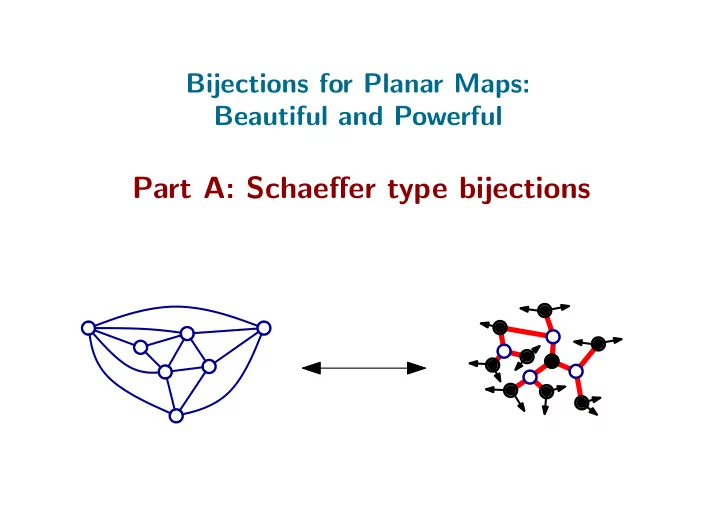
Part A: Schaeffer type bijections

Reminders about trees and maps

A.I

Trees

• Def. A tree is a connected acyclic graph.

Trees

• Def. A tree is a connected acyclic graph.
• Def. A rooted tree is a tree with a marked root-vertex.

parent, children, ancestors, descendants.

Trees

• Def. A tree is a connected acyclic graph.
• Def. A rooted plane tree is a rooted tree + order for children of

each vertex.

• Def. A rooted tree is a tree with a marked root-vertex.

parent, children, ancestors, descendants.

Trees

• Def. A tree is a connected acyclic graph.
• Def. A rooted plane tree is a rooted tree + order for children of

each vertex.

• Def. A rooted tree is a tree with a marked root-vertex.
• Remark. Rooted plane tree ⇐

⇒ rooted planar map with a single face. parent, children, ancestors, descendants.

Bijection for trees: contour code, height code, children code v0 v1 v2 v3 v4 v5 v6 v7 v8

n edges rooted plane tree

Bijection for trees: contour code, height code, children code v0 v1 v2 v3 v4 v5 contour code

height while making tour of the tree

v6 v7 v8

n edges

2n steps ±1. Stays ≥ 0, ends at 0.

rooted plane tree

Bijection for trees: contour code, height code, children code v0 v1 v2 v3 v4 v5 contour code height code

height of vi height while making tour of the tree

v6 v7 v8

n edges

2n steps ±1. Stays ≥ 0, ends at 0. n steps ≤ 1. Stays > 0 after 1st step.

rooted plane tree

Bijection for trees: contour code, height code, children code v0 v1 v2 v3 v4 v5 contour code height code children code

height of vi #children of vi -1 height while making tour of the tree

v6 v7 v8

n edges

2n steps ±1. Stays ≥ 0, ends at 0. n steps ≤ 1. Stays > 0 after 1st step. n+1 steps ≥ −

• 1. Stays ≥ 0 before ending at -1.

rooted plane tree

Bijection for trees: contour code, height code, children code v0 v1 v2 v3 v4 v5 contour code height code children code

height of vi #children of vi -1 height while making tour of the tree

v6 v7 v8

n edges

2n steps ±1. Stays ≥ 0, ends at 0. n steps ≤ 1. Stays > 0 after 1st step. n+1 steps ≥ −

• 1. Stays ≥ 0 before ending at -1.

Catn =

(2n)! n!(n+1)! trees

rooted plane tree

Euler formula

• Lemma. A tree satisfies

#edges = #vertices − 1.

Euler formula

• Lemma. A tree satisfies

#edges = #vertices − 1. More generally, a planar map sastisfies the Euler formula: #edges = #vertices + #faces − 2.

Duality

• Def. The dual of a planar map M is the map M ∗ obtained by

M

Duality

• Def. The dual of a planar map M is the map M ∗ obtained by

M M ∗

• drawing a vertex of M ∗ in each face of M,
• drawing an edge of M ∗ across each edge of M.

Duality between height code and children code height code children code children code height code

A fundamental toolkit for maps: spanning trees and orientations

A.II

Spanning tree

• Def. A spanning tree is an acyclic connected (spanning) subgraph.

Spanning tree

• Def. A spanning tree is an acyclic connected (spanning) subgraph.
• Remark. The dual of a spanning tree of M is a spanning tree of M ∗.

T T ∗

Spanning tree

• Def. A spanning tree is an acyclic connected (spanning) subgraph.
• Remark. The dual of a spanning tree of M is a spanning tree of M ∗.

T T ∗

T acyclic ← → T ∗ connected T connected ← → T ∗ acyclic

Minimal accessible orientations

• Def. An orientation is
• minimal if it has no counterclockwise directed cycle.
• accessible if every vertex is reachable from the root-vertex.

Minimal accessible orientations

• Def. An orientation is
• minimal if it has no counterclockwise directed cycle.

Example. accessible? minimal?

? ? ? ? ? ?

• accessible if every vertex is reachable from the root-vertex.

Minimal accessible orientations

• Def. An orientation is
• minimal if it has no counterclockwise directed cycle.

Example. accessible? minimal?

No Yes Yes Yes No Yes

• accessible if every vertex is reachable from the root-vertex.

Minimal accessible orientations

• Def. An orientation is
• minimal if it has no counterclockwise directed cycle.
• Remark. The dual of a minimal accessible orientation is . . .

O

• accessible if every vertex is reachable from the root-vertex.

Minimal accessible orientations

• Def. An orientation is
• minimal if it has no counterclockwise directed cycle.

O

• accessible if every vertex is reachable from the root-vertex.

O∗

• Remark. The dual of a minimal accessible orientation is a minimal

accessible orientation. O minimal ← → O∗ accessible O accessible ← → O∗ minimal

Minimal accessible orientations

• Def. An orientation is
• minimal if it has no counterclockwise directed cycle.

Remark.

• minimal orientations ←

→ cycle systems (equivalence class of

• rientations up to flipping directed cycles)
• accessible orientations ←

→ cocycle systems (equivalence class

• f orientations up to flipping directed cocycles)
• minimal accessible orientations ←

→ cycle-cocycle systems

• accessible if every vertex is reachable from the root-vertex.

• Def. Given a spanning tree T, we consider the counterclockwise tour.

Bijection 1: spanning trees ← → minimal accessible orientations

• Def. Given a spanning tree T, we consider the counterclockwise tour.

Bijection 1: spanning trees ← → minimal accessible orientations

• Def. Define Φ(T) = orientation obtained by
• orienting every edge e ∈ T from parent to child,
• orienting every edge e /

∈ T “clockwise” (that is, such that head of e appears before tail during tour).

Φ

Thm [B. 07]: The mapping Φ is a bijection between spanning trees and minimal accessible orientations. Bijection 1: spanning trees ← → minimal accessible orientations

Φ

Example:

Proof:

• Φ(T) accessible (because tree is oriented from root to leaves).
• Φ(T) minimal (because Φ(T)∗ is accessible).

Proof:

• Φ is injective: we can recover the tree while making its tour.
• Φ(T) accessible (because tree is oriented from root to leaves).
• Φ(T) minimal (because Φ(T)∗ is accessible).

? ? ?

Proof:

• Φ is injective: we can recover the tree while making its tour.
• Φ(T) accessible (because tree is oriented from root to leaves).
• Φ(T) minimal (because Φ(T)∗ is accessible).

? ? ?

• Φ is surjective: the above procedure always produces a spanning

tree (the subgraph it produces is connected because orientation is accessible and is acyclic because orientation is minimal).

Bijection 2: minimal accessible orientated map ← → mobiles.

Bijection 2: minimal accessible orientated map ← → mobiles. Definition: Consider a minimal accessible orientated map. Make every vertex explode according to the following rule.

explosion

Bijection 2: minimal accessible orientated map ← → mobiles. Definition: Consider a minimal accessible orientated map. Make every vertex explode according to the following rule.

explosion

Example:

explosion

Bijection 2: minimal accessible orientated map ← → mobiles.

explosion

Lemma: Orientation is minimal accessible ⇐ ⇒ explosion gives a tree.

Bijection 2: minimal accessible orientated map ← → mobiles.

explosion

Lemma: Orientation is minimal accessible ⇐ ⇒ explosion gives a tree. Proof: For an edge e of the map, we consider the left-path =“leftmost path” ending at e. e . . .

Bijection 2: minimal accessible orientated map ← → mobiles.

explosion

Lemma: Orientation is minimal accessible ⇐ ⇒ explosion gives a tree. Proof: For an edge e of the map, we consider the left-path =“leftmost path” ending at e. e

• left-paths of map = oriented paths of exploded map.
• If orientation is minimal accessible, then every left-path ends at

the root vertex (cannot end elsewhere nor cycle).

• A badly oriented cycle or cocycle creates a “trap” for left-paths.

. . .

To a minimal accessible orientation, we associate a mobile with

• white vertices corresponding to the vertices of M,
• black vertices corresponding to the faces of M.

The mobile is obtained by a controlled explosion: Bijection 2: minimal accessible orientated map ← → mobiles.

controlled explosion

To a minimal accessible orientation, we associate a mobile with

• white vertices corresponding to the vertices of M,
• black vertices corresponding to the faces of M.

The mobile is obtained by a controlled explosion: Bijection 2: minimal accessible orientated map ← → mobiles.

controlled explosion controlled explosion

Example:

Bijection 2: minimal accessible orientated map ← → mobiles. Lemma: The mobile is a tree.

controlled explosion

Example:

Bijection 2: minimal accessible orientated map ← → mobiles. Lemma: The mobile is a tree.

controlled explosion

Example: Proof:

• If the oriented map M has n edges, then mobile has:

n + 1 edges (because the root creates an edge), n + 2 vertices (Euler formula).

• The mobile is connected (because every cycle of M was broken

by the explosion).

Bijection 2: minimal accessible orientated map ← → mobiles.

controlled explosion

Example: Lemma: No loss of information in separation of tree and mobile. Proof: kth vertex of tree is glued to kth white corner of mobile.

1 2 3 4 5 6 7 8 1 2 3 4 5 6 7 8

Bijection 2: minimal accessible orientated map ← → mobiles. Thm: [B. 07] The controlled explosion is a bijection between

• minimal accessible oriented maps with n edges,
• pairs of rooted plane trees with n and n + 1 edges.

tree of left-paths mobile Example:

Summary

map + minimal accessible orientation map + spanning tree mobile + tree of left-paths

Summary General scheme of Shaeffer type bijection (for a class of maps):

map + minimal accessible orientation map + spanning tree mobile + tree of left-paths

• 1. Identify a canonical minimal accessible orientation.
• 2. Associate spanning-tree + decoration or Mobile + decoration.

Summary General scheme of Shaeffer type bijection (for a class of maps):

map + minimal accessible orientation map + spanning tree mobile + tree of left-paths

• 1. Identify a canonical minimal accessible orientation.
• 2. Associate spanning-tree + decoration or Mobile + decoration.

The art is in finding a good canonical orientation: it should characterize the class of maps and lead to simple decorations.

Additional remarks

• 1. Tree of left-paths can be encoded by either children-code,

height-code, dual children-code . . .

1 2 1 2 2 3 children-code height-code dual children-code

Additional remarks

• 1. Tree of left-paths can be encoded by either children-code,

height-code, dual children-code . . .

• 2. The toolbox is self-dual.

dual orientation corresponds to dual spanning tree dual orientation gives same mobile and dual tree

Additional remarks

controlled explosion controlled explosion

• 1. Tree of left-paths can be encoded by either children-code,

height-code, dual children-code . . .

• 2. The toolbox is self-dual.

Additional remarks

• 1. Tree of left-paths can be encoded by either children-code,

height-code, dual children-code . . .

• 2. The toolbox is self-dual.
• 3. The toolbox has a nice extension to other orientations.

extends into a bijection

• rientations ←

→ subgraphs case of acyclic orientations with several sources [B. 08] arxiv:0612003

Additional remarks

• 1. Tree of left-paths can be encoded by either children-code,

height-code, dual children-code . . .

• 2. The toolbox is self-dual.
• 3. The toolbox has a nice extension to other orientations.
• 4. The toolbox has a nice extension to higher genus.

[B., Chapuy 10] arxiv:1001.1592

The Cori-Vauquelin/Schaeffer’s bijection as a specialization of the Tree-rooted map bijection

A.III

Quadrangulation

• Def. A quadrangulation is a map with faces of degree 4.

Quadrangulation

• Def. A quadrangulation is a map with faces of degree 4.
• Prop. A quadrangulation is bipartite.

Quadrangulation

• Def. A quadrangulation is a map with faces of degree 4.
• Prop. A quadrangulation is bipartite.
• Proof. Any face has even degree.

⇒ Any cycle has even length. ⇒ The map is bipartite.

Quadrangulation

• Def. A quadrangulation is a map with faces of degree 4.
• Prop. A quadrangulation is bipartite.
• Cor. The distance from root-vertex changes by ±1 across each edge

(never 0).

2 1 2 1 2 2 3

Geodesic orientation

• Def. Geodesic orientation= orient every edge away from root-vertex.

2 1 2 1 2 2 3

Geodesic orientation

• Def. Geodesic orientation= orient every edge away from root-vertex.

2 1 2 1 2 2 3

• Remark. The geodesic orientation is minimal accessible.

Mobile obtained from the geodesic orientation

2 1 2 1 2 2 3

Mobile obtained from the geodesic orientation

2 1 2 1 2 2 3

• Remark. Every black vertex of the mobile has degree 2.

(except for root-face)

Mobile obtained from the geodesic orientation

2 1 2 1 2 2 3

• Remark. Every black vertex of the mobile has degree 2.

(except for root-face)

• Remark. All the left-paths (in fact, all directed paths) are geodesics.

Hence, distance labels = height code of trees of left-paths.

Mobile obtained from the geodesic orientation

2 1 2 1 2 2 3 2 1 2 1 2 2 3

• Def. Well-labeled trees = tree with positive labels such that root

has label 1 and label differ by 0,1, or −1 along edges. Thm [Shaeffer 98]. The above construction is a bijection between quadrangulations (n vertices) and well-labeled trees (n − 1 vertices).

Additional remarks

• 1. The above construction extends to bipartite maps:

it recovers [Bouttier, Di Francesco, Guitter 04].

2 1 2 1 2 2 3 2 1 2 1 2 2 3

Additional remarks

• 1. The above construction extends to bipartite maps:

it recovers [Bouttier, Di Francesco, Guitter 04].

• 2. The above construction extends to higher genus surfaces

[Marcus Schaeffer 98/Chapuy Marcus Schaeffer 08]

The master bijection framework

A.IV

A few bijections

• Triangulations (2n faces)
• Quadrangulations (n faces)
• Bipartite maps (ni faces of degree 2i)

Loopless: 2n (n + 1)(2n + 1) 3n n

• Simple:

1 n(2n − 1) 4n − 2 n − 1

• General:

2 · 3n (n + 1)(n + 2) 2n n

• Simple:

2 n(n + 1) 3n n − 1

• 2 · ( i ni)!

(2 + (i − 1)ni)!

• i

1 ni! 2i − 1 i ni [Poulalhon, Schaeffer 06 Fusy, Poulalhon, Schaeffer 08] [Schaeffer 97, Schaeffer 98] [Schaeffer 98, Fusy 07] [Schaeffer 97, Bouttier, Di Francesco, Guitter 04] [Poulalhon, Schaeffer 02]

Degree of the faces

Girth 1 2 3 4

1 2 3 4 5

6 7 8 A few bijections

Goal: Find a master bijection for planar maps which unifies all known bijections (of red type).

Goal:

• 1. Define a master bijection between a class of oriented maps

and a class of decorated trees.

• 2. Define canonical orientations for maps in any class defined by

degree and girth constraints. Find a master bijection for planar maps which unifies all known bijections (of red type). Strategy:

Goal: Find a master bijection for planar maps which unifies all known bijections (of red type).

Goal: Find a master bijection for planar maps which unifies all known bijections (of red type). Alternative strategies:

• Bijections of the blue type [Albenque, Poulalhon 15]

Same orientation. Encodes the map by “spanning tree with buds”.

Goal: Find a master bijection for planar maps which unifies all known bijections (of red type). Alternative strategies:

• Bijections of the blue type [Albenque, Poulalhon 15]

Same orientation. Encodes the map by “spanning tree with buds”.

• Recursive decomposition by slices [Bouttier, Guitter 14]

Direct cutting of the map. Same orientation (?).

Oriented maps

external face external vertices

A plane map is a planar map with a distinguished “external face”.

Oriented maps Let O be the set of oriented plane maps such that:

• there is no counterclockwise directed cycle (minimal),
• internal vertices can be reached from external vertices (accessible),
• external vertices have indegree 1.

external face external vertices

A plane map is a planar map with a distinguished “external face”.

A mobile is a plane tree with vertices properly colored in black and white, together with buds (arrows) incident only to black vertices. Mobiles

Master bijection Mapping Φ for an oriented map in O:

• Return the external edges.
• Place a black vertex in each internal face.

Draw an edge/bud for each clockwise/counterclockwise edge.

• Erase the map.

Master bijection Theorem [B.,Fusy]: The mapping Φ is a bijection between the set O

• f oriented maps and the set of mobiles with more buds than edges.

Moreover, indegree of internal vertices ← → degree of white vertices degree of internal faces ← → degree of black vertices degree of external face ← → #buds - #edges

Canonical orientations

Goal:

Degree of faces

Girth 1 2 3 4

1 2 3 4 5

6 7 C= class of maps defined by girth constraints and degree constraints. We want to define a canonical orientation in O for each map in C C

How to define a canonical orientation? We consider a plane map M and want to define an orientation in O (orientations which are minimal + accessible + external indegree 1).

How to define a canonical orientation? We consider a plane map M and want to define an orientation in O (orientations which are minimal + accessible + external indegree 1). Fact 1: Let α be a function from the vertices of M to N. If there is an orientation of M with indegree α(v) for each vertex v, then there is unique minimal one. ⇒ Orientations in O can be defined by specifying the indegree α(v).

How to define a canonical orientation? We consider a plane map M and want to define an orientation in O (orientations which are minimal + accessible + external indegree 1). Fact 2: An orientation with indegree α(v) exists (and is accessible) if and only if

• v∈V

α(v) = |E|

• ∀U ⊂ V ,
• v∈U

α(v) ≥ |EU| (strict if there is an external vertex / ∈ U). Fact 1: Let α be a function from the vertices of M to N. If there is an orientation of M with indegree α(v) for each vertex v, then there is unique minimal one. ⇒ Orientations in O can be defined by specifying the indegree α(v).

How to define a canonical orientation? We consider a plane map M and want to define an orientation in O (orientations which are minimal + accessible + external indegree 1). Conclusion: For a map G, one can define an orientation in O by specifying an indegree function α such that:

• v∈V

α(v) = |E|,

• ∀ U ⊂ V ,
• v∈U

α(v) ≥ |EU| (strict if an external vertex / ∈ U),

• α(v) = 1 for every external vertex v.

How to define a canonical orientation? We consider a plane map M and want to define an orientation in O (orientations which are minimal + accessible + external indegree 1). Conclusion: For a map G, one can define an orientation in O by specifying an indegree function α such that:

• v∈V

α(v) = |E|,

• ∀ U ⊂ V ,
• v∈U

α(v) ≥ |EU| (strict if an external vertex / ∈ U),

• α(v) = 1 for every external vertex v.

Remark: Specifying indegrees is also convenient for master bijection: indegrees of internal vertices ← → degrees of white vertices.

Example: Simple triangulations

Degree of faces

Girth 1 2 3 4

1 2 3 4 5

6 7

Proof: The numbers v, e, f of vertices edges and faces satisfy:

• Incidence relation: 3f = 2e.
• Euler relation: v − e + f = 2.
• Example: Simple triangulations

Fact: A triangulation with n internal vertices has 3n internal edges.

Example: Simple triangulations Natural candidate for indegree function: α : v →

• 3 if v internal

1 if v external . Fact: A triangulation with n internal vertices has 3n internal edges. 1 1 1 3 3 3 3

Example: Simple triangulations New proof: Euler relation + the incidence relation ⇒ α satisfies:

v∈V α(v) = |E|,

• ∀ U ⊂ V ,

u∈U α(u) ≥ |EU| (strict if an external vertex /

∈ U),

• α(v) = 1 for every external vertex v.
• Thm.[Schnyder 89] A triangulation admits an orientation with indegree

function α if and only if it is simple.

Example: Simple triangulations Thm.[Schnyder 89] A triangulation admits an orientation with indegree function α if and only if it is simple.

• faces have degree 3
• internal vertices have indegree 3

⇒ The class of simple triangulations is identified with the class of

• riented maps in O such that

Example: Simple triangulations

• black vertices have degree 3
• white vertices have degree 3

Thm [recovering FuPoSc08]: The master bijection Φ induces a bijection between simple triangulations and mobiles such that Thm.[Schnyder 89] A triangulation admits an orientation with indegree function α if and only if it is simple.

• faces have degree 3
• internal vertices have indegree 3

⇒ The class of simple triangulations is identified with the class of

• riented maps in O such that

Example: Simple triangulations

• black vertices have degree 3
• white vertices have degree 3

Thm [recovering FuPoSc08]: The master bijection Φ induces a bijection between simple triangulations and mobiles such that Thm.[Schnyder 89] A triangulation admits an orientation with indegree function α if and only if it is simple.

• faces have degree 3
• internal vertices have indegree 3

⇒ The class of simple triangulations is identified with the class of

• riented maps in O such that

Corollary: The number of rooted simple triangulations with 2n faces is 1 n(2n − 1) 4n − 2 n − 1

• .

Orientations for d-angulations of girth d Fact: A d-angulation with (d−2)n internal vertices has dn internal edges. Natural candidate for indegree function: α : v →

• d/(d − 2) if v internal

1 if v external . . .

d = 5

Orientations for d-angulations of girth d Idea: We can look for an orientation of (d−2)G with indegree function α : v →

• d if v internal

1 if v external . Fact: A d-angulation with (d−2)n internal vertices has dn internal edges. 5 5 5 5 5 5 Natural candidate for indegree function: α : v →

• d/(d − 2) if v internal

1 if v external . . .

d = 5

Orientations for d-angulations of girth d 2 1 2 1 2 1 2 1 Thm [B., Fusy]: Let G be a d-angulation. G has girth d ← → G admits a weighted orientation with

• weight d − 2 per edges.
• ingoing weight d per internal vertex,
• ingoing weight 1 per external vertex.

i≤0 j >0 i>0 j >0 i+j = d−2

Orientations for d-angulations of girth d Proof: Use the Euler relation + incidence relation as before.

• 2

1 2 1 2 1 2 1 Thm [B., Fusy]: Let G be a d-angulation. G has girth d ← → G admits a weighted orientation with

• weight d − 2 per edges.
• ingoing weight d per internal vertex,
• ingoing weight 1 per external vertex.

Moreover, G admits a unique such orientation in O in this case.

i≤0 j >0 i>0 j >0 i+j = d−2

3 3 3 3 3 3 0

Orientations for maps of girth d

Degree of faces

Girth 1 2 3 4

1 2 3 4 5

6 7

Orientations for maps of girth d Thm [B., Fusy]: Let G be a map. G has girth d ← → G admits a weighted bi-orientation with

• weight d − 2 per edges.
• ingoing weight d per internal vertex,
• ingoing weight 1 per external vertex,
• clockwise outgoing weight d − deg per faces.

1 2 2 1 1 2 1 2 2 1

• 1

4 5

• 2
• 1

4

• 1 4

3 3 3 3 3 3 i≤0 j >0 i>0 j >0 i≤0 j ≤0 i+j = d−2

Moreover, G admits a unique such orientation in O in this case.

d = 5

Master bijection for weighted bi-orientation Theorem [B., Fusy] There is a bijection between weighted bi-oriented plane maps in O and weighted mobiles. Moreover, weight of internal edges ← → weight of edges ingoing weight of internal vertices ← → weight of white vertices degree of internal faces ← → degree of black vertices

• utgoing weight of internal faces ←

→ weight of black vertices

1 2 2 2 2 1 2 1 1 1

• 1

4 5

• 2
• 14
• 1

4 30 3 3 0 3 3 3 1 2 2 1 1 2 1 2 21

• 1

4 5

• 2
• 1

4

• 14

3 3 3 3 3 3

Canonical orientations + Master bijection

• edges have weight d − 2,
• white vertices have weight d,
• black vertices have weight d − deg.

Thm [B., Fusy]: There is a bijection between plane maps of girth d and weighted mobiles such that

1 2 2 2 2 1 2 1 1 1

• 1

4 5

• 2
• 14
• 1

4 30 3 3 0 3 3 3 12 21 1 2 1 2 21

• 1

4 5

• 2
• 1

4

• 14

3 3 3 3 3 3

Moreover, faces of degree d ← → black vertices of degree d.

Additional results and remarks

Distance?

• Remark. The buds of the mobile encodes the children code of the

dual tree of left-paths. Equivalently, they encode (the steps of) the height-code of the tree of left-paths, that is the left-path distance from the external face

Distance?

• Remark. The buds of the mobile encodes the children code of the

dual tree of left-paths. Equivalently, they encode (the steps of) the height-code of the tree of left-paths, that is the left-path distance from the external face [Addario-Berry, Albenque 2017] The left-path distance is close to the geodesic distance with high probabity.

Bijections for planar maps Master bijection approach covers

• Classes of maps defined by girth constraint + degree constraints.

Degree of the faces

Girth 1 2 3 4

1 2 3 4 5

6

[FuPoSc08] [Sc98] [Sc97,BoDiGu02] [PoSc02]

7 8

Bijections for planar maps Master bijection approach covers

• Classes of maps defined by girth constraint + degree constraints.
• Case d = 0 [Schaeffer 98, Bouttier, Di Francesco, Guitter 04].

Degree of the faces

Girth 1 2 3 4

1 2 3 4 5

6

[FuPoSc08] [Sc98] [Sc97,BoDiGu02] [PoSc02]

7 8

[Sc98,BoDiGu04]

Bijections for planar maps Master bijection approach covers

• Classes of maps defined by girth constraint + degree constraints.
• Case d = 0 [Schaeffer 98, Bouttier, Di Francesco, Guitter 04].
• d-angulations with non-facial girth at least d, generalizing [Fusy,

Poulalhon, Schaeffer 08,Fusy 09].

Degree of the faces

Girth 1 2 3 4

1 2 3 4 5

6

[FuPoSc08] [Sc98] [Sc97,BoDiGu02] [PoSc02]

7 8

[Sc98,BoDiGu04]

Bijections for maps with boundaries Master bijection approach extends to maps with boundaries. [B., Fusy 18]

Bijections for hypermaps Master bijection approach extends to hypermaps. [B., Fusy 19]

Bijections for hypermaps Master bijection approach extends to hypermaps. The master bijection generalizes bijections by [Bousquet-M´ elou, Schaeffer 00] (Constellations), [Bousquet-M´ elou, Schaeffer 02] (Ising model), [Bouttier, Di Francesco, Guitter 04] (Distances). [B., Fusy 19]

More fun with girth constraints? +2 +1 |C| ≥ d +

• f inside C

σ(f) In [B. Fusy] we introduce “charges” as a tool to control more general cycle-length constraints. Question: Can we prove new probabilistic results on the cycle lengths in random maps?

End of part A.

Main references (for this part of the minicourse):

• Conjugaison d’arbres et cartes combinatoires al´

eatoires [Scha- effer 98]

• Bijective counting of tree-rooted maps and shuffles of paren-

thesis systems [Bernardi 07]

• A bijection for covered maps, or a shortcut between Harer-

Zagier’s and Jackson’s formulas [Bernardi, Chapuy 11]

• A bijection for triangulations, quadrangulations, pentagula-

tions, etc [Bernardi, Fusy 12]

• Unified bijections for maps with prescribed degrees and girth

[Bernardi, Fusy 12]

Bonus: Counting Thm[B., Fusy]: d-angulations of girth d. The generating function Fd(x) =

• d-angulation
• f girth d

x#faces is given by Fd(x) = Wd−2 −

d−3

• i=0

WiWd−2−i, and F ′

d(x) = (1 + W0)d,

where W0, W1, . . . , Wd−2 are defined by:

• ∀j < d − 2,

Wj =

• r
• i1,...,ir>0

i1+···+ir=j+2

Wi1 · · · Wir,

• Wd−2 = x(1 + W0)d−1.

Bonus: Counting Thm[B., Fusy]: d-angulations of girth d. The generating function Fd(x) =

• d-angulation
• f girth d

x#faces is given by Fd(x) = Wd−2 −

d−3

• i=0

WiWd−2−i, and F ′

d(x) = (1 + W0)d,

where W0, W1, . . . , Wd−2 are defined by:

• ∀j < d − 2,

Wj =

• r
• i1,...,ir>0

i1+···+ir=j+2

Wi1 · · · Wir,

• Wd−2 = x(1 + W0)d−1.

Example d=5: W0 = W 2

1 + W2

W1 = W 3

1 + 2W1W2 + W3

W2 = W 4

1 + 3W 2 1 W2 + 2W1W3 + W 2 2

W3 = x(1 + W0)4

Bonus: Counting Thm[B., Fusy]: Maps of girth d (having outer degree d). The generating function Fd(xd, xd

+ 1, ..)=

• maps of

girth d

• i

x#faces of deg i

i

is given by Fd = Wd−2 −

d−3

• j=−2

WjWd−2−j where ∀j ∈ [−2..d−3], Wj =

• r
• i1,...,ir>0

i1+···+ir=j+2

Wi1 · · · Wir, and ∀j ∈ [d−2..d], Wj = [uj+1]

• i

xi (u + uW0 + W−1 + u−1)i−1.

Extends case d = 1 [Bouttier, Di Francesco, Guitter 02]

Bonus: Counting Thm[B., Fusy]: Maps of girth d (having outer degree d). The generating function Fd(xd, xd

+ 1, ..)=

• maps of

girth d

• i

x#faces of deg i

i

is given by Fd = Wd−2 −

d−3

• j=−2

WjWd−2−j where ∀j ∈ [−2..d−3], Wj =

• r
• i1,...,ir>0

i1+···+ir=j+2

Wi1 · · · Wir, and ∀j ∈ [d−2..d], Wj = [uj+1]

• i

xi (u + uW0 + W−1 + u−1)i−1. Corollaries: If the set of admissible face degrees is finite, then

• Algebraic generating function.
• Asymptotic number of maps: ∼ c n−5/2 ρn.

Extends case d = 1 [Bouttier, Di Francesco, Guitter 02] Extends case d=1 [Bender, Canfield 94]