A new combinatorial identity for unicellular maps, via a direct - - PowerPoint PPT Presentation

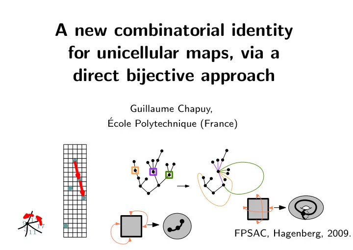
FPSAC, Hagenberg, 2009. Guillaume Chapuy,

A new combinatorial identity for unicellular maps, via a direct bijective approach

3 9 11 13 17

´ Ecole Polytechnique (France)

Unicellular maps as polygon gluings We start with a 2n-gon, and we paste the edges pairwise in order to form an orientable surface.

Unicellular maps as polygon gluings We start with a 2n-gon, and we paste the edges pairwise in order to form an orientable surface.

Unicellular maps as polygon gluings We start with a 2n-gon, and we paste the edges pairwise in order to form an orientable surface.

Unicellular maps as polygon gluings We start with a 2n-gon, and we paste the edges pairwise in order to form an orientable surface.

Unicellular maps as polygon gluings We start with a 2n-gon, and we paste the edges pairwise in order to form an orientable surface. The image of the polygon forms the drawing of an n-edge graph on the surface. Euler’s formula relates the number of vertices to the genus of the surface : v = n + 1 − 2g

Unicellular maps as polygon gluings We start with a 2n-gon, and we paste the edges pairwise in order to form an orientable surface. The image of the polygon forms the drawing of an n-edge graph on the surface. 1 vertex, genus 1 3 vertices, genus 0 Euler’s formula relates the number of vertices to the genus of the surface : v = n + 1 − 2g

Unicellular maps as polygon gluings We start with a 2n-gon, and we paste the edges pairwise in order to form an orientable surface. The image of the polygon forms the drawing of an n-edge graph on the surface. 1 vertex, genus 1 3 vertices, genus 0 Euler’s formula relates the number of vertices to the genus of the surface : v = n + 1 − 2g

Counting Aim: count unicellular maps of fixed genus. The number of unicellular maps with n edges is equal to the number

• f distinct matchings of the edges : (2n)!

2nn! .

Counting Aim: count unicellular maps of fixed genus. The number of unicellular maps with n edges is equal to the number

• f distinct matchings of the edges : (2n)!

2nn! . For instance, in the planar case... Unicellular maps are exactly plane trees. Therefore the number of n-edge unicellular maps of genus 0 is : ǫ0(n) = Cat(n) = 1 n + 1 2n n

Higher genus ? For each g the number of n-edge unicellular maps of genus g has the (beautiful) form : ǫg(n) = (some polynomial) × Cat(n) ǫ1(n) = (n+1)n(n−1)

12

Cat(n) ǫ2(n) = (n+1)n(n−1)(n−2)(n−3)(5n−2)

1440

Cat(n) For instance : References : Lehman and Walsh 72 (formal power series), Harer and Zagier 86 (matrix integrals).

Higher genus ? For each g the number of n-edge unicellular maps of genus g has the (beautiful) form : ǫg(n) = (some polynomial) × Cat(n) ǫ1(n) = (n+1)n(n−1)

12

Cat(n) ǫ2(n) = (n+1)n(n−1)(n−2)(n−3)(5n−2)

1440

Cat(n) For instance : References : Lehman and Walsh 72 (formal power series), Harer and Zagier 86 (matrix integrals). No combinatorial interpretation !

Higher genus ? For each g the number of n-edge unicellular maps of genus g has the (beautiful) form : ǫg(n) = (some polynomial) × Cat(n) ǫ1(n) = (n+1)n(n−1)

12

Cat(n) ǫ2(n) = (n+1)n(n−1)(n−2)(n−3)(5n−2)

1440

Cat(n) For instance : References : Lehman and Walsh 72 (formal power series), Harer and Zagier 86 (matrix integrals). No combinatorial interpretation ! Note for experts: the Goulden-Nica bijection does not solve the same problem (it solves a ”Poissonized” version of the problem).

Map = graph + rotation system = All the information is contained in the pair formed by the graph and the cyclic ordering of edges around each vertex.

Map = graph + rotation system = All the information is contained in the pair formed by the graph and the cyclic ordering of edges around each vertex. We started from one single polygon ⇒ the graph has only one border

Map = graph + rotation system = All the information is contained in the pair formed by the graph and the cyclic ordering of edges around each vertex. We started from one single polygon ⇒ the graph has only one border

Map = graph + rotation system = All the information is contained in the pair formed by the graph and the cyclic ordering of edges around each vertex. We started from one single polygon ⇒ the graph has only one border

Map = graph + rotation system = All the information is contained in the pair formed by the graph and the cyclic ordering of edges around each vertex. We started from one single polygon ⇒ the graph has only one border

Map = graph + rotation system = All the information is contained in the pair formed by the graph and the cyclic ordering of edges around each vertex. We started from one single polygon ⇒ the graph has only one border

Map = graph + rotation system = All the information is contained in the pair formed by the graph and the cyclic ordering of edges around each vertex. We started from one single polygon ⇒ the graph has only one border

= To do: cut the 2g independant cycles of this graph in order to obtain a tree. Problem: where to cut ? All the information is contained in the pair formed by the graph and the cyclic ordering of edges aroud each vertex. We started from one single polygon ⇒ the graph has only one border Map = graph + rotation system

Numbering the corners. We follow the border of the map starting from the root, and we number the corners from 1 to 2n.

Numbering the corners. We follow the border of the map starting from the root, and we number the corners from 1 to 2n.

1 2 3 border

Numbering the corners. We follow the border of the map starting from the root, and we number the corners from 1 to 2n.

1 2 3 4 border 5 6 8 7 9 10

Numbering the corners. We follow the border of the map starting from the root, and we number the corners from 1 to 2n.

1 2 3 4 border 5 6 8 7 9 10 11 12 13 14 15 16 17 18 19 20

Numbering the corners. We follow the border of the map starting from the root, and we number the corners from 1 to 2n.

1 2 3 4 border 5 6 8 7 9 10 11 12 13 14 15 16 17 18 19 20 3 9 11 13 17

We compare the two natural orderings of corners around one vertex: this gives a diagram.

Numbering the corners. We follow the border of the map starting from the root, and we number the corners from 1 to 2n.

1 2 3 4 border 5 6 8 7 9 10 11 12 13 14 15 16 17 18 19 20 3 9 11 13 17

1 2

. . .

20

We compare the two natural orderings of corners around one vertex: this gives a diagram.

Planar case In the planar case, the border-numbering and the cyclic ordering always coincide:

Planar case In the planar case, the border-numbering and the cyclic ordering always coincide:

1st 2nd 3rd 4th

For each vertex, the diagram is increasing:

Planar case In the planar case, the border-numbering and the cyclic ordering always coincide:

1st 2nd 3rd 4th

For each vertex, the diagram is increasing: Higher genus Around each vertex, a decrease in the diagram is called a trisection.

3 9 11 13 17

1 2

. . .

20 trisection trisection

The trisection lemma A unicellular map of genus g always has exactly 2g trisections. → It is an equivalent problem to count unicellular maps with a distinguished trisection. Proof: simple counting argument.

How to build a trisection : first method.

• Start with a map of genus (g − 1) with three marked vertices.
• Let a1 < a2 < a3 be the labels of their minimal corners.

a1 a2 a3

• Glue these three corners together as follows :

How to build a trisection : first method.

• Start with a map of genus (g − 1) with three marked vertices.
• Let a1 < a2 < a3 be the labels of their minimal corners.

a1 a2 a3

• Glue these three corners together as follows :

How to build a trisection : first method.

• Start with a map of genus (g − 1) with three marked vertices.
• Let a1 < a2 < a3 be the labels of their minimal corners.

a1 a2 a3

• Glue these three corners together as follows :

How to build a trisection : first method.

• Start with a map of genus (g − 1) with three marked vertices.
• Let a1 < a2 < a3 be the labels of their minimal corners.

a1 a2 a3

• Glue these three corners together as follows :

How to build a trisection : first method.

• Start with a map of genus (g − 1) with three marked vertices.
• Let a1 < a2 < a3 be the labels of their minimal corners.

a1 a2 a3

• Glue these three corners together as follows :

How to build a trisection : first method.

• Start with a map of genus (g − 1) with three marked vertices.
• Let a1 < a2 < a3 be the labels of their minimal corners.

a1 a2 a3

• Glue these three corners together as follows :

How to build a trisection : first method.

• Start with a map of genus (g − 1) with three marked vertices.
• Let a1 < a2 < a3 be the labels of their minimal corners.

a1 a2 a3

• Glue these three corners together as follows :

1 → 2 → . . . → a3 → → a2 → → a1 → . . . → 2n . . . . . .

• The resulting map has only one border :

How to build a trisection : first method.

• Start with a map of genus (g − 1) with three marked vertices.
• Let a1 < a2 < a3 be the labels of their minimal corners.

a1 a2 a3

• Glue these three corners together as follows :

1 → 2 → . . . → a3 → → a2 → → a1 → . . . → 2n . . . . . .

• The resulting map has only one border :

1

1

How to build a trisection : first method.

• Start with a map of genus (g − 1) with three marked vertices.
• Let a1 < a2 < a3 be the labels of their minimal corners.

a1 a2 a3

• Glue these three corners together as follows :

1 → 2 → . . . → a3 → → a2 → → a1 → . . . → 2n . . . . . .

• The resulting map has only one border :

1 2

1 2

How to build a trisection : first method.

• Start with a map of genus (g − 1) with three marked vertices.
• Let a1 < a2 < a3 be the labels of their minimal corners.

a1 a2 a3

• Glue these three corners together as follows :

1 → 2 → . . . → a3 → → a2 → → a1 → . . . → 2n . . . . . .

• The resulting map has only one border :

3 1 2

1 2 3

a1 a2 a3 1 → 2 → . . . → a3 → → a2 → → a1 → . . . → 2n . . . . . .

3 1 2

1 2 3

How to build a trisection : first method.

• Start with a map of genus (g − 1) with three marked vertices.
• Let a1 < a2 < a3 be the labels of their minimal corners.
• The resulting map has only one border :
• Glue these three corners together as follows :

a1 a2 a3 1 → 2 → . . . → a3 → → a2 → → a1 → . . . → 2n . . . . . .

3 1 2

1 2 3

• By Euler’s formula, it has genus g.

How to build a trisection : first method.

• Start with a map of genus (g − 1) with three marked vertices.
• Let a1 < a2 < a3 be the labels of their minimal corners.
• The resulting map has only one border :
• Glue these three corners together as follows :

a1 a2 a3 1 → 2 → . . . → a3 → → a2 → → a1 → . . . → 2n . . . . . .

3 1 2

1 2 3

• By Euler’s formula, it has genus g.
• Moreover we have built a trisection.

trisection

How to build a trisection : first method.

• Start with a map of genus (g − 1) with three marked vertices.
• Let a1 < a2 < a3 be the labels of their minimal corners.
• The resulting map has only one border :
• Glue these three corners together as follows :

Therefore we have a mapping : a1 a2 a3 genus g − 1, three marked vertices genus g, one marked trisection

Therefore we have a mapping : a1 a2 a3 genus g − 1, three marked vertices genus g, one marked trisection The mapping is injective because we can retrieve the three cor- ners, and cut the vertex back.

Therefore we have a mapping : a1 a2 a3 genus g − 1, three marked vertices genus g, one marked trisection The mapping is injective because we can retrieve the three cor- ners, and cut the vertex back.

1 : minimum corner

Therefore we have a mapping : a1 a2 a3 genus g − 1, three marked vertices genus g, one marked trisection The mapping is injective because we can retrieve the three cor- ners, and cut the vertex back.

1 : minimum corner 2: corner following the marked trisection

Therefore we have a mapping : a1 a2 a3 genus g − 1, three marked vertices genus g, one marked trisection The mapping is injective because we can retrieve the three cor- ners, and cut the vertex back.

1 : minimum corner 2: corner following the marked trisection 3: smallest corner be- tween 2 and 1 which is greater than 2

Therefore we have a mapping : a1 a2 a3 genus g − 1, three marked vertices genus g, one marked trisection The mapping is injective because we can retrieve the three cor- ners, and cut the vertex back.

1 : minimum corner 2: corner following the marked trisection 3: smallest corner be- tween 2 and 1 which is greater than 2

Hence : 2g · ǫg(n) = n + 3 − 2g 3

• ǫg−1(n) + . . .

genus g marked trisection genus g − 1 3 marked vertices

Therefore we have a mapping : a1 a2 a3 genus g − 1, three marked vertices genus g, one marked trisection The mapping is injective because we can retrieve the three cor- ners, and cut the vertex back.

1 : minimum corner 2: corner following the marked trisection 3: smallest corner be- tween 2 and 1 which is greater than 2

Hence : 2g · ǫg(n) = n + 3 − 2g 3

• ǫg−1(n) + . . .

genus g marked trisection genus g − 1 3 marked vertices

?

Let’s try the reverse mapping... genus g marked trisection

Let’s try the reverse mapping... genus g marked trisection

1 : minimum corner

Let’s try the reverse mapping... genus g marked trisection

1 : minimum corner 2: corner following the marked trisection

Let’s try the reverse mapping... genus g marked trisection

3: smallest corner be- tween 2 and 1 which is greater than 2 1 : minimum corner 2: corner following the marked trisection

Let’s try the reverse mapping... a1 a2 a3 genus g − 1, three marked corners genus g marked trisection

3: smallest corner be- tween 2 and 1 which is greater than 2 1 : minimum corner 2: corner following the marked trisection

Let’s try the reverse mapping... a1 a2 a3 genus g − 1, three marked corners

• We still have a1 < a2 < a3 in the map of genus (g − 1).

genus g marked trisection

3: smallest corner be- tween 2 and 1 which is greater than 2 1 : minimum corner 2: corner following the marked trisection

Let’s try the reverse mapping... a1 a2 a3 genus g − 1, three marked corners

• We still have a1 < a2 < a3 in the map of genus (g − 1).
• a1 and a2 are both the minimum corner in their vertex.

genus g marked trisection

3: smallest corner be- tween 2 and 1 which is greater than 2 1 : minimum corner 2: corner following the marked trisection

Let’s try the reverse mapping... a1 a2 a3 genus g − 1, three marked corners

• We still have a1 < a2 < a3 in the map of genus (g − 1).
• a1 and a2 are both the minimum corner in their vertex.
• This is not always the case for a3 :

genus g marked trisection

3: smallest corner be- tween 2 and 1 which is greater than 2 1 : minimum corner 2: corner following the marked trisection

Let’s try the reverse mapping... a1 a2 a3 genus g − 1, three marked corners

• We still have a1 < a2 < a3 in the map of genus (g − 1).
• a1 and a2 are both the minimum corner in their vertex.
• This is not always the case for a3 :
• If a3 is the minimum of its vertex : we are in the image of the

previous construction. genus g marked trisection

3: smallest corner be- tween 2 and 1 which is greater than 2 1 : minimum corner 2: corner following the marked trisection

Let’s try the reverse mapping... a1 a2 a3 genus g − 1, three marked corners

• We still have a1 < a2 < a3 in the map of genus (g − 1).
• a1 and a2 are both the minimum corner in their vertex.
• This is not always the case for a3 :
• If a3 is the minimum of its vertex : we are in the image of the

previous construction.

• Else a3 is incident to a trisection of the map of genus (g − 1).

genus g marked trisection

3: smallest corner be- tween 2 and 1 which is greater than 2 1 : minimum corner 2: corner following the marked trisection

Therefore : genus g, one marked trisection genus (g − 1), 3 marked vertices genus (g − 1), 2 vertices and 1 trisection

good case bad case

Therefore : genus g, one marked trisection genus (g − 1), 3 marked vertices genus (g − 1), 2 vertices and 1 trisection genus (g − 2), 2+3=5 marked vertices genus (g − 2), 2+2=4 vertices and 1 trisection distinguished

good case bad case good case bad case good case bad case

and so on...

Our main result: genus g,

• ne marked trisection = ∪

i > 0 genus g−i and 2i+1 marked vertices.

( )

bij.

Our main result: genus g,

• ne marked trisection = ∪

i > 0 genus g−i and 2i+1 marked vertices.

( )

bij.

2g ·ǫg(n) n+3−2g

3

• ǫg−1(n)+

= And a new formula:

Our main result: genus g,

• ne marked trisection = ∪

i > 0 genus g−i and 2i+1 marked vertices.

( )

bij.

2g ·ǫg(n) n+3−2g

3

• ǫg−1(n)+n+5−2g

5

• ǫg−2(n)+

= And a new formula:

Our main result: genus g,

• ne marked trisection = ∪

i > 0 genus g−i and 2i+1 marked vertices.

( )

bij.

2g ·ǫg(n) n+3−2g

3

• ǫg−1(n)+n+5−2g

5

• ǫg−2(n)+

. . . + n+1

2g+1

• Cat(n)

= And a new formula:

Our main result: genus g,

• ne marked trisection = ∪

i > 0 genus g−i and 2i+1 marked vertices.

( )

bij.

2g ·ǫg(n) n+3−2g

3

• ǫg−1(n)+n+5−2g

5

• ǫg−2(n)+

. . . + n+1

2g+1

• Cat(n)

= ǫg(n) = (some polynomial) × Cat(n)

• = ”number” of possibilities for the

successive choices of vertices. And a new formula: =

• 0=g0<g1<...<gr=g

r

• i=1

1 2gi n + 1 − 2gi−1 2(gi − gi−1) + 1

• Everything boils down to plane trees:

For instance : 2 · ǫ1(n) = (n+1)n(n−1)

6

Cat(n)

For instance : 2 · ǫ1(n) = (n+1)n(n−1)

6

Cat(n) 4 · ǫ2(n) = (n−1)(n−2)(n−3)

6

ǫ1(n) + (n+1)n(n−1)(n−2)(n−3)

5!

Cat(n) = (n+1)n(n−1)(n−2)(n−3)(5n−2)

1440

Cat(n)

Extensions

• The formula leads to a differential equation which enables to re-

cover the known closed formulas for the generating functions (Harer- Zagier, Itzykson-Zuber).

• Works the same for bipartite unicellular maps.
• The Marcus-Schaeffer bijection relates general maps on surfaces

to labelled unicellular maps. The composition of the two bijections leads to a description of general maps of given genus in terms of labelled trees with distinguished vertices. This gives information about the continuum limit of maps on surfaces (Brownian map of genus g).

Thank you!

(n+1)ǫg(n) = 2(2n−1)ǫg(n−1)+(2n−1)(n−1)(2n−3)ǫg−1(n−2) R´ ecurrence :

• g≥0

ǫg(n)yn+1−2g = (2n)! 2nn!

• i≥1

2i−1 n i − 1 y i

• Version sommatoire :

Formules d’Harer et Zagier :