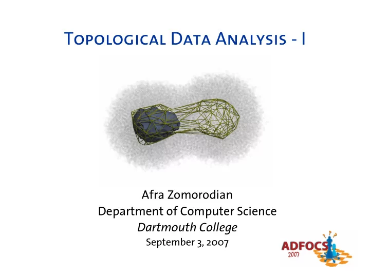
Topological Data Analysis - I Afra Zomorodian Department of - PowerPoint PPT Presentation

Topological Data Analysis - I Afra Zomorodian Department of Computer Science Dartmouth College September 3, 2007 1

Acquisition • Vision: Images (2D) • GIS: Terrains (3D) • Graphics: Surfaces (3D) • Medicine: MRI (Volumetric 3D) 2

Simulation • Folding @ Home – ~1M CPUs, ~200K active – ~200 Tflops sustained performance – [Kasson et al. ‘06] 3

Abstract Spaces • Spaces with motion • Each point in abstract space is a snapshot • Robotics: Configuration spaces (nD) • Biology: Conformation spaces (nD) 4

A Thought Exercise • Example: 1 x 10 6 points in 100 dimensions • How to compress? – Gzip? – Zip? – Better? • Arbitrary compression not possible • Knowledge: Points are on a circle – Fit a circle, parameterize it – Store angles ( ≈ 100x compression) – Run Gzip • Insight: Knowledge of structure allows compression • Topology deals with structure 5

Computational Topology • My view • Input: Point Cloud Data – Massive – Discrete – Nonuniformly Sampled – Noisy – Embedded in R d , sometimes d >> 3 • Mission: What is its shape? 6

Plan • Today: ☺ Motivation – Topology – Simplicial Complexes – Invariants – Homology – Algebraic Complexes • Tomorrow – Geometric Complexes – Persistent Homology – The Persistence Algorithm – Application to Natural Images 7

Outline ☺ Motivation • Topology – Topological Space – Manifolds – Erlanger Programm – Classification • Simplicial Complexes • Invariants • Homology • Algebraic Complexes 8

Topological Space • X: set of points • Open set: subset of X Topology: set of open sets T ⊆ 2 X such that • 1. If S 1 , S 2 ∈ T, then S 1 ∩ S 2 ∈ T 2. If {S J | j ∈ T}, then ∪ j ∈ J S j ∈ T 3. ∅ , X ∈ T X = (X, T) is a topological space • • Note: different topologies possible • Metric space: open sets defined by metric 9

Homeomorphism • Topological spaces X , Y • Map f : X → Y • f is continuous, 1-1, onto (bijective) • f -1 also continuous • f is a homeomorphism X is homeomorphic to Y • X ≈ Y • X and Y have same topological type • 10

Examples interval ≈ S 1 • Closed interval • S 1 ≈ Figure 8 • S 1 ≈ Annulus 1 Circle S • • Annulus ≈ B 2 • S 2 ≈ Cube • Figure 8 • • Captures – boundary • Annulus – junctions – holes Ball B 2 • – dimension Sphere S 2 • • Continuous ⇒ no gluing Continuous -1 ⇒ no tearing • • Cube • Stretching allowed! 11

Erlanger Programm 1872 • Christian Felix Klein (1849-1925) • Unifying definition: 1. Transform space in a fixed way 2. Observe properties that do not change • Transformations – Rigid motions: translations & rotations – Homeomorphism: stretch, but do not tear or sew • Rigid motions ⇒ Euclidean Geometry • Homeomorphisms ⇒ Topology 12

Geometry vs. Topology • Euclidean geometry – What does a space look like? – Quantitative – Local – Low-level – Fine • Topology – How is a space connected? – Qualitative – Global – High-level – Coarse 13

The Homeomorphism Problem • Given: topological spaces X and Y • Question: Are they homeomorphic? • Much coarser than geometry – Cannot capture singular points (edges, corners) – Cannot capture size – Classification system 14

Manifolds • Given X S 1 • Every point x ∈ X has neighborhood ≈ R d ( X is separable and Hausdorff) • S 2 X is a d-manifold (d-dimensional) • X has some points with nbhd ≈ H d = {x ∈ R d | x 1 ≥ 0} • X is a d-manifold with boundary • • Boundary ∂ X are those points 15

Compact 2-Manifolds S 1 • d = 1: one manifold S 2 • d = 2: orientable . . . Torus Double Torus Triple Torus . . . • d = 2: non-orientable Projective Plane P 2 Klein Bottle 16

Manifold Classification • Compact manifolds – closed – bounded • d = 1: Easy • d = 2: Done [Late 1800’s] • d ≥ 4: Undecidable [Markov 1958] – Dehn’s Word Problem 1912 – [Adyan 1955] • d = 3: Very hard – The Poincaré Conjecture 1904 – Thurston’s Geometrization Program 1982: piece-wise uniform geometry – Ricci flow with surgery [Perelman ’03] 17

Outline ☺ Motivation ☺ Topology • Simplicial Complexes – Geometric Definition – Combinatorial Definition • Invariants • Homology • Algebraic Complexes 18

Simplices • Simplex: convex hull of affinely independent points • 0-simplex: vertex • 1-simplex: edge • 2-simplex: triangle • 3-simplex: tetrahedron • k-simplex: k + 1 points • face of simplex σ : defined by subset of vertices • Simplicial complex: glue simplices along shared faces 19

Simplicial Complex • Every face of a simplex in a complex is in the complex Edge is missing • Non-empty intersection of two simplices is a face of each of them Sharing half an edge Intersection not a vertex 20

Abstract Simplicial Complex • Set of sets S such that if A ∈ S , so is every subset of A c f • S = { ∅ , e d b {a}, {b}, {a, b}, {c}, {b, c}, a {d}, {c, d}, {e}, {d, e}, {f}, g {e, f}, {g}, {d, g}, {e, g}, h {d, e, g}, {h}, {d, h}, {e, h}, m {g, h}, {d, g, h}, {d, e, h}, {e, g, h}, i {d, e, g, h}, {i}, {h, i}, {j}, {i, j}, {k}, k l {i, k}, {j, k}, {i, j, k}, {l}, {k, l}, {m}, {a, m}, {b, m}, {l, m} j } Geometric Visualization Abstract Geometric Vertex Scheme 21

Outline ☺ Motivation ☺ Topology ☺ Simplicial Complexes • Invariants – Definition – The Euler Characteristic – Homotopy • Homology • Algebraic Complexes 22

Invariants • The Homeomorphism problem is hard • How about a partial answer? • Topological invariant: a map f that assigns the same object to spaces of the same topological type – X ≈ Y ⇒ f( X ) = f( Y ) – f( X ) ≠ f( Y ) ⇒ X ≈ Y (contrapositive) – f( X ) = f( Y ) ⇒ nothing • Spectrum f( X ) = one object, for all X – trivial: f( X ) = f( Y ) ⇒ X ≈ Y – complete: 23

The Euler Characteristic • Given: (abstract) simplicial complex K • s i : # of i-simplices in K • Euler characteristic ξ (K): ξ (torus) = 9 – 27 + 18 = 0 24

The Euler Characteristic • Invariant, so complex does not matter ξ (sphere) = 2 • ξ (tetrahedron) = 4 – 6 + 4 = 2 – ξ (cube) = 8 – 12 + 6 = 2 – ξ (disk ∪ point) = 1 – 0 + 1 = 2 – ξ (g-torus) = 2 – 2g, genus g • ξ (g P 2 ) = 2 – g • 25

Homotopy • Given: Family of maps f t : X → Y , t ∈ [0,1] • Define F : X × [0,1] → Y , F(x,t) = f t (x) 1 F 0 X Y • If F is continuous, f t is a homotopy • f 0 , f 1 : X → Y are homotopic via f t • f 0 ' f 1 26

Homotopy Equivalence • Given: f : X → Y • Suppose ∃ g : Y → X such that A – f o g ' 1 Y – g o f ' 1 X • f is a homotopy equivalence • X and Y are homotopy equivalent X ' Y • Comparison – Homeomorphism: g o f = 1 X f o g = 1 Y – Homotopy: g o f ' 1 X f o g ' 1 Y (Theorem) X ≈ Y ⇒ X ' Y • (Theorem) • Contractible: homotopy equivalent to a point 27

Outline ☺ Motivation ☺ Topology ☺ Simplicial Complexes ☺ Invariants • Homology – Intuition – Homology Groups – Computation – Euler-Poincaré • Algebraic Complexes 28

Intuition 29

Overview • Algebraic topology: algebraic images of topological spaces • Homology – How cells of dimension n attach to cells of dimension n – 1 – Images are groups, modules, and vector spaces • Simplicial homology: cells are simplices • Plan: – chains: like paths, maybe disconnected – cycles: like loops, but a loop can have multiple components – boundary: a cycle that bounds 30

Chains • Given: Simplicial complex K • k-chain: – list of k-simplices in K – formal sum ∑ i n i σ i , where n i ∈ {0, 1} and σ i ∈ K • Field Z 2 – 0 + 0 = 0 – 0 + 1 = 1 + 0 = 1 – 1 + 1 = 0 • Chain vector space C k : vector space spanned by k-simplices in K • rank C k = s k , number of k-simplices in K 31

Boundary Operator ∂ k : C k → C k-1 • • homomorphism (linear) σ = [v 0 , ..., v k ] • ∂ k σ = ∑ i [v 0 , …, v i 0 , …, v k ], • 0 indicates that v i is deleted from the sequence where v i ∂ 1 ab = a + b • ∂ ∂ 2 abc = ab + bc + ac • ∂ 1 ∂ 2 abc = a + b + b + c + a + c = 0 • ∂ • (Theorem) ∂ k-1 ∂ k = 0 for all k 32

Cycles • Let c be a k-chain • If c has no boundary, it is a k-cycle ∂ k c = 0, so c ∈ ker ∂ k • • Z k = ker ∂ k is a subspace of C k ∂ 1 (ab + bc + ac) = • a + b + b + c + a + c = 0, so 1-chain ab + bc + ac is a 1-cycle 33

Boundaries • Let b be a k-chain • If b bounds something, it is a k-boundary ∃ d ∈ C k+1 such that b = ∂ k+1 d • • B k = im ∂ k+1 is a subspace of C k ∂ 2 (abc) = ab + bc + ac, • so ab + bc + ac is a 1-boundary ∂ k b = ∂ k ∂ k+1 d = 0, so b is also a k-cycle! • • All boundaries are cycles • B k ⊆ Z k ⊆ C k 34

Homology Group • The kth homology vector space (group) is H k = Z k / B k = ker ∂ k / im ∂ k+1 (Theorem) X ' Y ⇒ H k ( X ) ≅ H k ( Y ) • (Theorem) • If z 1 = z 2 + b, where b ∈ B k , z 1 and z 2 are homologous, z 1 ∼ z 2 z 2 z 1 35