EVC Computer Vision R h Rehersal 1 l 1 http:// - - PowerPoint PPT Presentation

EVC ‐ Computer Vision

R h l 1 Rehersal 1

http://www.caa.tuwien.ac.at/cvl/teaching/sommersemester/evc

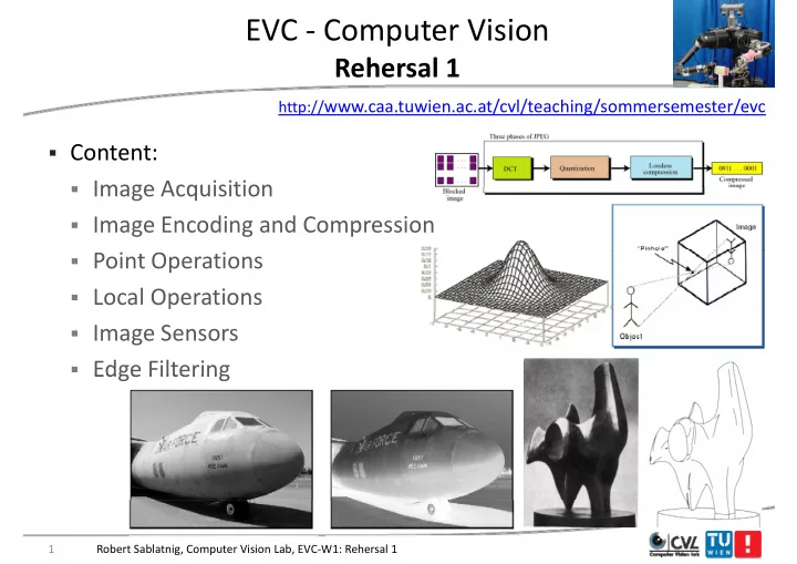
• Content:
• Image Acquisition
• Image Acquisition
• Image Encoding and Compression
• Point Operations
• Local Operations
• Image Sensors
• Edge Filtering

Edge Filtering

1 Robert Sablatnig, Computer Vision Lab, EVC‐W1: Rehersal 1

Human Eye y

2 Robert Sablatnig, Computer Vision Lab, EVC‐W1: Rehersal 1

Human Eye ‐ Components y p

• Cornea + Lens:
• Light fraction
• Light fraction
• Iris:

i bl t

• variable aperture
• Retina: Image Detector
• (ca. 100 Mio.

Photoreceptors)

3 Robert Sablatnig, Computer Vision Lab, EVC‐W1: Rehersal 1

Retina

• Rods:

Monochrome

• Cones:

Color (RGB)

• Cones:

Color (RGB)

• Fovea:

Cones only N b 6 Mi C

• Number:

6 Mio. Cones 120 Mio. Rods

• But only 1

1 Mio. nerve fibers

• Mio. nerve fibers in
• ptic nerve => intelligent

intelligent ! sensor sensor!

Robert Sablatnig, Computer Vision Lab, EVC‐W1: Rehersal 1 4

The Plenoptic Function p

Adelson & Bergen, 91 The intensity P can be parameterized as:

Image coordinates (sperical)

The intensity P can be parameterized as:

P ( t,  Vx, Vy, Vz)

“Th l t t f ll i t tit t th t ibiliti f i i ”

(sperical) Color Time 3D space

“The complete set of all convergence points constitutes the permanent possibilities of vision.” Gibson

5 Robert Sablatnig, Computer Vision Lab, EVC‐W1: Rehersal 1

Measuring the Plenoptic Function g p

Why is there no picture appearing on the paper?

Robert Sablatnig, Computer Vision Lab, EVC‐W1: Rehersal 1 6

Why is there no picture appearing on the paper?

Measuring the Plenoptic Function g p

The camera obscura The pinhole camera

Robert Sablatnig, Computer Vision Lab, EVC‐W1: Rehersal 1 7

Image Geometry g y

• Simplest Model: Pinhole camera

p

• Has a very small hole

(Aperture = ∞), Light is led (Aperture ), Light is led through the hole and forms an image at the back of the g box (upside down and side‐ inverted)

8 Robert Sablatnig, Computer Vision Lab, EVC‐W1: Rehersal 1

Image Geometry g y

• Perspective Projection (Central projection)
• Is the projection of the 3d world onto a 2d plane by rays passing
• Is the projection of the 3d world onto a 2d plane by rays passing

through a common point the center of projection.

• => models image formation by a pinhole camera
• => models image formation by a pinhole camera

9 Robert Sablatnig, Computer Vision Lab, EVC‐W1: Rehersal 1

Equations of the perspective projection q p p p j

f f x X Z f x  Z f X x  Y f y  f y  Y Z y Z Y

• Perspective projection is non‐linear !

10 Robert Sablatnig, Computer Vision Lab, EVC‐W1: Rehersal 1

Recap: Limits of Pinhole Cameras p

• A picture of a filament taken with a pinhole camera. In the image
• n the left, the hole was too big (blurring), and in the image on

, g ( g), g the right, the hole was too small (diffraction).

Ruechardt, 1958

11 Robert Sablatnig, Computer Vision Lab, EVC‐W1: Rehersal 1

Simple Lens Parameters p

u v u v

12 Robert Sablatnig, Computer Vision Lab, EVC‐W1: Rehersal 1

Lenses

Pi h l ll A t f li ht

• Pin has no lens => small Aperture => few light
• „thin" lenses: small Aperture but much light
• Thin lens law:

u y  v yi  f y  f v yi  

13 Robert Sablatnig, Computer Vision Lab, EVC‐W1: Rehersal 1

Lenses

• f: focal length = distance of the point on

the optical axis where all rays emerging p y g g from infinity meet to the lens plane ( = all rays are parallel to the optical axis) y p p )

• if u = ∞ then v = f
• Rays going through the optical center of
• Rays going through the optical center of

the lens are not diffracted

• Field of view: area that is recorded by a

1 1 1

• Field of view: area that is recorded by a

camera: Th bi f th ll th th t i

f v u 1 1 1  

• The bigger f the smaller the area that is

imaged d l ll f l f

f

• Wide‐angle ‐ small f; Zoom ‐ large f

14 Robert Sablatnig, Computer Vision Lab, EVC‐W1: Rehersal 1

Depth of Field p

• Only objects in a certain distance are imaged sharply at the image

plane, all other distances are blurred because of blur circles. p ,

• The bigger the aperture, the bigger the blur circles
• The smaller the aperture the sharper is the image
• The smaller the aperture, the sharper is the image

 The bigger the depth of

field the darker the image

 Large Aperture = small

depth of field p

15 Robert Sablatnig, Computer Vision Lab, EVC‐W1: Rehersal 1

Depth of Field p

16 Robert Sablatnig, Computer Vision Lab, EVC‐W1: Rehersal 1

Different numbers of Gray Levels y

17 Robert Sablatnig, Computer Vision Lab, EVC‐W1: Rehersal 1

Radiometric Resolution

• Number of digital values (“gray levels”) that a sensor can use to

express variability of signal (“brightness”) within the data p y g ( g )

• Determines the information content of the image
• The more digital values the more detail can be expressed
• The more digital values, the more detail can be expressed
• Determined by the number of bits of within which the digital

information is encoded information is encoded 21 = 2 levels (0,1) 2² = 4 levels (0,1,2,3) 28 = 256 levels (0‐255) 212 = 4096 levels (0‐4095)

18 Robert Sablatnig, Computer Vision Lab, EVC‐W1: Rehersal 1

How many gray levels are required? y g y q

• Contouring is most visible for a ramp
• Digital images typically are quantized to 256 gray levels.

Transition to a Digital Image ‐ 1 g g

20 Robert Sablatnig, Computer Vision Lab, EVC‐W1: Rehersal 1

Transition to a Digital Image ‐ 2 g g

21 Robert Sablatnig, Computer Vision Lab, EVC‐W1: Rehersal 1

Image Size and Resolution g

• These images were produced by simply picking every n‐th sample

horizontally and vertically and replicating that value nxn times: y y p g

22 Robert Sablatnig, Computer Vision Lab, EVC‐W1: Rehersal 1

Sampling Theorem p g

h h h h i f i i Shannon Theorem Shannon Theorem: Exact reconstruction of a continuous‐time baseband signal from its samples is possible if the signal is b dli it d d th li f li f i t th t th t i t i bandlimited and the sampling frequency sampling frequency is greater than greater than twice twice the signal bandwidth the signal bandwidth.

y y x y x Abtastsignal x abzutastendes Signal abzutastendes Signal abgetastetes Signal

23 Robert Sablatnig, Computer Vision Lab, EVC‐W1: Rehersal 1

Image Sensors g

• Convert light into electric charge

CCD (charge coupled device) CMOS (complementary metal CCD (charge coupled device) Higher dynamic range High uniformity CMOS (complementary metal

Oxide semiconductor)

Lower voltage High uniformity Lower noise g Higher speed Lower system complexity y p y

24 Robert Sablatnig, Computer Vision Lab, EVC‐W1: Rehersal 1

Chromatic Aberration

longitudinal chromatic aberration transverse chromatic aberration (axial) (lateral)

25 Robert Sablatnig, Computer Vision Lab, EVC‐W1: Rehersal 1

Spherical Aberration p

• Effect: sharp image

superimposed by a blurred one

• Caused by spherical lens

surfaces (manufacturing)

• Parallel rays are focused in one

point only if they are close to h i l i the optical axis

• Can be avoided by using

h i l l ith aspherical lenses with parabolic surfaces

26 Robert Sablatnig, Computer Vision Lab, EVC‐W1: Rehersal 1

Geometric Lens Distortions

Radial distortion Tangential distortion

Photo by Helmut Dersch

Both due to lens imperfection

Photo by Helmut Dersch

27 Robert Sablatnig, Computer Vision Lab, EVC‐W1: Rehersal 1

How CCDs Record Color

Robert Sablatnig, Computer Vision Lab, EVC‐W1: Rehersal 1 28

Bayer Filter y

29 Robert Sablatnig, Computer Vision Lab, EVC‐W1: Rehersal 1

Goal of Image Compression g p

• Digital images require huge amounts of space for storage and

large bandwidths for transmission. g

• A 640 x 480 color image requires close to 1MB of space.
• The goal of image compression is to reduce the amount of data
• The goal of image compression is to reduce the amount of data

required to represent a digital image. Red ce storage req irements and increase transmission rates

• Reduce storage requirements and increase transmission rates.

30 Robert Sablatnig, Computer Vision Lab, EVC‐W1: Rehersal 1

Data Compression p

l d ll b f

• Data compression implies sending or storing a smaller number of

bits.

• lossless and
• lossy methods.
• Trade‐off: image quality vs compression ratio

31 Robert Sablatnig, Computer Vision Lab, EVC‐W1: Rehersal 1

Run Length Encoding (RLE) g g ( )

• Simplest method of compression
• Can be used to compress data made of any combination of
• Can be used to compress data made of any combination of

symbols, does not need to know the frequency of occurrence of symbols symbols

• Replace consecutive repeating occurrences of a symbol by one
• ccurrence of the symbol followed by the number of occurrences
• ccurrence of the symbol followed by the number of occurrences

Original 2 3 4 6 3 Original Coded

• Lossless compression!

p

Robert Sablatnig, Computer Vision Lab, EVC‐W1: Rehersal 1 32

Huffman Encoding

• Character code found by starting at the root and following the

branches that lead to that character.

• The code itself is the bit value of each branch on the path, taken

in sequence.

• Decoding: reverse process
• Decoding: reverse process

Robert Sablatnig, Computer Vision Lab, EVC‐W1: Rehersal 1 33

JPEG Compression p

• Image is divided into blocks of 8 × 8 pixel blocks to decrease the

number of calculations because the number of mathematical

• perations for each image is the square of the number of units.

34 Robert Sablatnig, Computer Vision Lab, EVC‐W1: Rehersal 1

JPEG Compression p

• Idea: change image into a linear (vector) set of numbers that

reveals redundancies.

• Redundancies can be removed using one of the lossless

compression methods compression methods

Robert Sablatnig, Computer Vision Lab, EVC‐W1: Rehersal 1 35

JPEG Compression p

8 pixels s An 8x8 block 8 pixels DCT Quantiser Entropy Encoder Channel zigzag Image IDCT Dequantiser Entropy Decoder Channel

• r

Storage reverse zigzag

• To perform the JPEG coding, an image (in color or grey scales) is first

subdivided into blocks of 8x8 pixels subdivided into blocks of 8x8 pixels.

• The Discrete Cosine Transform (DCT) is then performed on each block.
• This generates 64 coefficients which are then quantized to reduce their

g q magnitude.

Robert Sablatnig, Computer Vision Lab, EVC‐W1: Rehersal 1 36

JPEG Compression p

8 pixels s An 8x8 block 8 pixels DCT Quantiser Entropy Encoder Channel zigzag Image IDCT Dequantiser Entropy Decoder Channel

• r

Storage reverse zigzag

• The coefficients are then reordered into a one‐dimensional array in a

zigzag manner before further entropy encoding zigzag manner before further entropy encoding.

• The compression is achieved in two stages; the first is during

quantization and the second during the entropy coding process.

• JPEG decoding is the reverse process of coding.

Robert Sablatnig, Computer Vision Lab, EVC‐W1: Rehersal 1 37

Videocompression p

• Single Image
• Size 720 x 576 px
• Size 720 x 576 px
• Pixelresolution: 1 Byte/RGB Value

→ 720 576 3 (B t ) 1 215 KB → 720 x 576 x 3 (Byte) ~ 1.215 KB

• Image sequence
• 25 fps

→ 720 x 576 x 25 x 3 (Byte) ~ 30.375 KB/s ( y ) /

38 Robert Sablatnig, Computer Vision Lab, EVC‐W1: Rehersal 1

M‐ JPEG

• Videosequenzes
• Single image compression using JPEG
• Single image compression using JPEG

…..

JPEG- Kompression

Benefits Drawbacks

Constant Image Quality Fluctuating bandwidth / frame rate Fast computation High memory requirements Robust with respect to packet loss No Audio

39 Robert Sablatnig, Computer Vision Lab, EVC‐W1: Rehersal 1

Types of Operations yp p

• The operations that can be applied to digital images to transform

an input image a[m,n] into an output image b[m,n] p g [ , ] p g [ , ]

• Point: the output value at a specific coordinate is dependent
• nly on the input value at that same coordinate.
• nly on the input value at that same coordinate.
• Local: the output value at a specific coordinate is dependent on

the input values in the neighborhood of that same coordinate the input values in the neighborhood of that same coordinate

• Global: the output value at a specific coordinate is dependent
• n all the values in the input image
• n all the values in the input image

40 Robert Sablatnig, Computer Vision Lab, EVC‐W1: Rehersal 1

Point Operations p

• Point Operations perform a mapping of the pixel values without

changing the size, geometry, or local structure of the image g g , g y, g

• Each new pixel value I’(u,v) depends on the previous value I(u,v)

at the same position and on a mapping function f() at the same position and on a mapping function f()

• The function f() is independent of the coordinates

S ch operation is called “homogeneo s”

• Such operation is called “homogeneous”

41 Robert Sablatnig, Computer Vision Lab, EVC‐W1: Rehersal 1

Threshold Operation p

• Thresholding an image is a special type of quantization that

separates the pixel values in two classes, depending on a given p p , p g g threshold value pth

• The threshold function maps all the pixels to one of two fixed

The threshold function maps all the pixels to one of two fixed intensity values po, p1 0 < pth ≤ pmax

• Example: binarization: po=0, p1=1

42 Robert Sablatnig, Computer Vision Lab, EVC‐W1: Rehersal 1

Histogram g

• Assume that the digital image has q discrete gray levels and that

nk, k = 0, ..., q‐1, is the number of pixel having intensity k. The histogram is given by:

n r h r p

k k k

  ) ( ) (

where p is the normalized histogram function, n the total number

n n

• f image pixels. nk are the number of pixels in the bin assigned to

pixels with intensity level k.

• It gives a measure of how likely is for a pixel to have a certain
• intensity. That is, it gives the probability of occurrence the

intensity intensity.

• The sum of the normalized histogram function over the range of

all intensities is 1 all intensities is 1.

Robert Sablatnig, Computer Vision Lab, EVC‐W1: Rehersal 1 43

Histogram g

• The histogram function can be plotted
• graphically. The image histogram carries

g p y g g important information about the image content.

Robert Sablatnig, Computer Vision Lab, EVC‐W1: Rehersal 1 44

Histogram Normalization g

• Goal: utilization of the

complete gray level range p g y g

• => linear spreading of gray
• => linear spreading of gray

levels to the complete gray level range

• riginal

level range ) ( I

min max min

) , ( ) , ( ' q q q v u I q v u I    

stretched

45 Robert Sablatnig, Computer Vision Lab, EVC‐W1: Rehersal 1

Histogram Equalization g q

Let r(x y) be a gray level image whose minimum intensity value is r and

• Let r(x,y) be a gray‐level image whose minimum intensity value is rmin and

maximum intensity value rmax. The dynamic range of the image ∆r is: ∆r = rmax‐ rmin.

• The Probability Function (PF) of the image r(x,y) is p(r = a) = pr(a). With a

probability of pr(a) the image takes a gray‐level equal to the value of a.

• Histogram equalization means that we need to find a intensity level
• Histogram equalization means that we need to find a intensity level

transforming function T(a) that for the transformed image r‘(x,y) can be computed as

)) ( ( ) ( ' y x r T y x r 

• T(a) is chosen in way that the probability function pr‘ (a) of the

transformed image r‘(x,y) has a predefined shape.

)) , ( ( ) , ( y x r T y x r 

transformed image r (x,y) has a predefined shape.

pr(a) pr‘ (a)

46 Robert Sablatnig, Computer Vision Lab, EVC‐W1: Rehersal 1

Histogram Equalization Example g q p

Original

• Goal: Equal Distribution
• f gray levels over the

Original g y complete gray level range g

• => Contrast is enhanced

at maxima and a a a a d weakened at minima Equalized

47 Robert Sablatnig, Computer Vision Lab, EVC‐W1: Rehersal 1

Local‐Operators p

The Gray level of the resulting pixel is dependent on several pixel in the The Gray level of the resulting pixel is dependent on several pixel in the

• riginal image:
• An operator window is placed around an actual pixel

p p p

• Computation of the resulting pixel by combination of gray levels of

the actual pixel and its neighbors and saving it at the position of the actual pixel at its position in the result image actual pixel at its position in the result image

• Computation of the complete image (by displacement of the operator

window by one pixel)

Operator window Operator window Actual pixel

48 Robert Sablatnig, Computer Vision Lab, EVC‐W1: Rehersal 1

Linear 2‐D Filter

49 Robert Sablatnig, Computer Vision Lab, EVC‐W1: Rehersal 1

Smoothing Spatial Filtering g p g

Origin x

1/9 1/9 1/9 1/9 1/9 1/9

O igin x

104 100 108 99 106 98 *

/9 /9 /9

1/9 1/9 1/9

99 106 98 95 90 85 *

Filter

Simple 3*3 Neighbourhood

106

104 99 95 100 108 98 90 85

1/9 1/9 1/9 1/9 1/9 1/9 1/9 1/9 1/9

3*3 Smoothing Filter

Original Image Pixels

e = 1/9*106 +

1/9*104 + 1/9*100 + 1/9*108 +

95 90 85

/9 /9 /9

y Image f (x, y)

1/9*99 + 1/9*98 + 1/9*95 + 1/9*90 + 1/9*85 9 9 9

= 98.3333

The above is repeated for every pixel in the original image to generate p y p g g g the smoothed image

50 Robert Sablatnig, Computer Vision Lab, EVC‐W1: Rehersal 1

Strange Things Happen At The Edges! g g pp g

At the edges of an image we are missing pixels to form a At the edges of an image we are missing pixels to form a neighbourhood

Origin Origin x

e e e e e e e e

Robert Sablatnig, Computer Vision Lab, EVC‐W1: Rehersal 1 51

y Image f (x, y)

Two‐dimensional Convolution

Function Function Function Function

Linerar Linerar Convolution

52 Robert Sablatnig, Computer Vision Lab, EVC‐W1: Rehersal 1

Properties of linear Filters p

• Commutative:
• I

H = H I

• I H = H I
• Linear:

( I) H I ( H) (I H)

• (a ∙ I) H = I (a ∙ H) = a ∙ (I H)
• (I1 + I2) H = (I1

H) + (I2 H)

• Associative:
• A (B C) = (A B) C

( ) ( )

• Separabel: H = H1

H2 . . . Hn

Robert Sablatnig, Computer Vision Lab, EVC‐W1: Rehersal 1 53

Image Filters g

• Filter kernels are scaled in order to guarantee that the brightness

does not change generally. The scaling factor is computed by the g g y g p y sum of the coefficients of the kernel matrix.

• Example:

Example:

 Intensity of a pixel is the sum of all of its 8

neighbors

 On a white image (all pixel = 1) new value 9!  Intensity of a pixel is the average of all of its 8

y p g neighbors

 On a white image (all pixel = 1) new value 1!

g ( p )

54 Robert Sablatnig, Computer Vision Lab, EVC‐W1: Rehersal 1

Gaussian Filter

• Filter kernel can be approximated by convolution of two one‐

dimensional binomial distributions.

A i ti t G ‘ b ll h (2D) Approximation to Gauss‘ bell‐shape curve (2D) Example: 3x3 Gaussian Kernel

55 Robert Sablatnig, Computer Vision Lab, EVC‐W1: Rehersal 1

Gaussian Filter

• Gaussians are used because:
• Smooth (infinitely differentiable)
• Smooth (infinitely differentiable)
• Decay to zero rapidly

Si l l ti f l

• Simple analytic formula
• Separable: multidimensional Gaussian = product of Gaussians in

each dimension

• Convolution of 2 Gaussians = Gaussian
• Limit of applying multiple filters is Gaussian (Central limit

theorem)

56 Robert Sablatnig, Computer Vision Lab, EVC‐W1: Rehersal 1

Non‐linear Filters

• Linear filters may have disadvantages: Linear smoothing filter

suppresses noise but blurs the image at the same time. pp g

• Non‐linear filters (rank value filters) do not have this
• disadvantage. Therefore they are usually applied for noise
• disadvantage. Therefore they are usually applied for noise

removal.

57 Robert Sablatnig, Computer Vision Lab, EVC‐W1: Rehersal 1

Median Filter

The Median filter is a non‐linear

• filter. The kernel window selects a

pixel set S around the center coordinates (xc,yc) of the original

• image. The new value C‘(xc,yc) is set

h di l f h i l to the median value of the pixel set

• S. That is C‘(xc,yc) = median( S ).

58 Robert Sablatnig, Computer Vision Lab, EVC‐W1: Rehersal 1

Median Filter: Outliers are eliminated

59 Robert Sablatnig, Computer Vision Lab, EVC‐W1: Rehersal 1

Edge Detection g

• Edges describe colloquially the edge of a surface or a significant

change in orientation of the surface normals N l Normals Texture Depth

60 Robert Sablatnig, Computer Vision Lab, EVC‐W1: Rehersal 1

Types of Edges yp g

• Step and "roof" edges
• Direction (positive or negative)

Direction (positive or negative)

• Difference between gray values

along an edge Contrast Contrast along an edge: Contrast Contrast

• Discontinuities

Discontinuities of the brightness represent: Discontinuities of surface normal normal Discontinuities of the depth depth Discontinuities of texture texture Discontinuities of illumination illumination

61 Robert Sablatnig, Computer Vision Lab, EVC‐W1: Rehersal 1

Edge‐derivative g

Profile of one image line g Gradient Magnitude

62 Robert Sablatnig, Computer Vision Lab, EVC‐W1: Rehersal 1

What happens at an edge? pp g

Bright

Positive Edge

image region

Gradient is high!

1st Derivative

63 Robert Sablatnig, Computer Vision Lab, EVC‐W1: Rehersal 1

How to measure the 1st Derivative?

for discrete signals only approximation possible

64 Robert Sablatnig, Computer Vision Lab, EVC‐W1: Rehersal 1

Simple horizontal Contour Filter p

65 Robert Sablatnig, Computer Vision Lab, EVC‐W1: Rehersal 1

Goal: Find Edges independent of their Orientation g p

• Method by Roberts (1965)

66 Robert Sablatnig, Computer Vision Lab, EVC‐W1: Rehersal 1

Image Gradient g

• The gradient of an image:
• The gradient points in the direction of most rapid increase in

i i intensity

• The edge strength is given by the gradient magnitude:

67 Robert Sablatnig, Computer Vision Lab, EVC‐W1: Rehersal 1

Image Gradient g

• The gradient points in the direction of most rapid increase in

intensity intensity

• The gradient of a surface at a point defines the tangential plane

to the surface at this point to the surface at this point h d thi l t t th di ti f th d ?

• how does this relate to the direction of the edge?

68 Robert Sablatnig, Computer Vision Lab, EVC‐W1: Rehersal 1

Sobel Filter

• Less noise dependent than Robert’s (due to bigger filter size)

69 Robert Sablatnig, Computer Vision Lab, EVC‐W1: Rehersal 1

Roberts vs. Sobel Operator p

70 Robert Sablatnig, Computer Vision Lab, EVC‐W1: Rehersal 1

Related Operators p

x  y    1 x    1 y      1 1 x      1 1 1 y         1 1       1 1          1 1 1 1            1 1 1

2x2 Roberts

    1 1     1 1 1

3x3 Prewitt   1 2 1 y    1 1 x 

    3 3 3 3 y        3 1 1 3 x 

      1 2 1         2 2 1 1

            1 1 1 1 1 1 1 1             3 1 1 3 3 1 1 3

         1 2 1       1 1 3 3 S b l

          3 3 3 3 1 1 1 1         3 1 1 3 3 1 1 3

4 4 P itt

Robert Sablatnig, Computer Vision Lab, EVC‐13: Local Operations – Edge Filtering 71

3x3 Sobel 4x4 Prewitt

Kirsch‐Operator (1971) p ( )

• Additional filters (different orientations)
• Less orientation dependent than Sobel‐Operator
• Less orientation dependent than Sobel Operator

No square root! „Compass“ Operator

72 Robert Sablatnig, Computer Vision Lab, EVC‐W1: Rehersal 1

Zero Crossing

T ti t th iti f th d i l th To estimate the position of the edge more precisely the zero crossing of the 2nd derivative is determined

73 Robert Sablatnig, Computer Vision Lab, EVC‐W1: Rehersal 1

Laplace Filter p

• Mathematical approximation of second derivative. Drawback: not

not directional anymore! directional anymore! y

• Because of the high pass characteristics (2nd order filter = 2nd

derivative) the Laplace filter is very sensitive to noise very sensitive to noise.

• Therefore it is rarely applied alone. Usually it is combined with a

Gaussian Filter that reduces noise before the Laplace filter can be applied.

74 Robert Sablatnig, Computer Vision Lab, EVC‐W1: Rehersal 1

Laplace of Gaussian (LoG) p ( )

C bi ti f G i Filt G i Filt d L l Filt L l Filt

• Combination of Gaussian Filter

Gaussian Filter and Laplace Filter Laplace Filter

• Combination corresponds to second derivative of the 2D Gaussian

function Laplacian of Gaussian filter (LoG): function Laplacian of Gaussian filter (LoG):

• Because of the shape of its kernel elements the LoG filter is

usually called “Mexican Hat

Mexican Hat” filter

y

• LoG Filter can be used for Edge Detection
• LoG Filter does

does not depend not depend on a particular direction. p

p

75 Robert Sablatnig, Computer Vision Lab, EVC‐W1: Rehersal 1

Canny Edge Detector y g

MATLAB: edge(image,‘canny’)

1.

Filter image with derivative of Gaussian

MATLAB: edge(image, canny )

1.

Filter image with derivative of Gaussian Fi d it d d i t ti f di t

2.

Find magnitude and orientation of gradient

3.

Non‐maximum suppression

4.

Linking and thresholding (hysteresis):

• Define two thresholds: low and high
• Use the high threshold to start edge curves and

h l h h ld i h the low threshold to continue them

76 Robert Sablatnig, Computer Vision Lab, EVC‐W1: Rehersal 1

Example p

Sobel Sobel Canny LOG

77 Robert Sablatnig, Computer Vision Lab, EVC‐W1: Rehersal 1

From Edgels to Edges g g

Contour Tracing Find Strucures (Lines, Circles)

78 Robert Sablatnig, Computer Vision Lab, EVC‐W1: Rehersal 1