Top Volume 11, Number 2, 151-228 December 2003 REPRINT M. - - PDF document

▶

Oct 28, 2023 236 likes •1.07k views

Top Volume 11, Number 2, 151-228 December 2003 REPRINT M. Guignard Lagrangean Relaxation A.J. Conejo (comment) 200 J. Desrosiers (comment)

SLIDE 1

Top

Volume 11, Number 2, 151-228 December 2003

REPRINT

M. Guignard

Lagrangean Relaxation

A.J. Conejo (comment) 200

J. Desrosiers (comment) 204

L.F. Escudero (comment) 206

A. Frangioni (comment) 215
A. Lucena (comment) 219
M. Guignard (rejoinder) 224

Published by Sociedad de Estadística e Investigación Operativa Madrid, Spain

SLIDE 2

Top

Volume 11, Number 2 December 2003

Editors Marco A. LÓPEZ-CERDÁ Ignacio GARCÍA-JURADO

Technical Editor Antonio ALONSO-AYUSO

Associate Editors

Ramón ÁLVAREZ-VALDÉS Nelson MACULAN Julián ARAOZ J.E. MARTÍNEZ-LEGAZ Jesús ARTALEJO Jacqueline MORGAN Jaume BARCELÓ Marcel NEUTS Emilio CARRIZOSA Fioravante PATRONE Eduardo CASAS Blas PELEGRÍN Laureano ESCUDERO Frank PLASTRIA Simon FRENCH Francisco J. PRIETO Miguel A. GOBERNA Justo PUERTO Monique GUIGNARD Gerhard REINELT Horst HAMACHER David RÍOS-INSUA Onésimo HERNÁNDEZ-LERMA Carlos ROMERO Carmen HERRERO Juan TEJADA Joaquim JÚDICE Stef TIJS Kristiaan KERSTENS Andrés WEINTRAUB Published by Sociedad de Estadística e Investigación Operativa Madrid, Spain

SLIDE 3

Sociedad de Estad´ ıstica e Investigaci´

n Operativa

Top (2003) Vol. 11, No. 2, pp. 151–228

Lagrangean Relaxation

Monique Guignard

Operations and Information Management Department The Wharton School, University of Pennsylvania E-mail: guignard@wharton.upenn.edu

Abstract

This paper reviews some of the most intriguing results and questions related to La- grangean relaxation. It recalls essential properties of the Lagrangean relaxation and

f the Lagrangean function, describes several algorithms to solve the Lagrangean

dual problem, and considers Lagrangean heuristics, ad-hoc or generic, because these are an integral part of any Lagrangean approximation scheme. It discusses schemes that can potentially improve the Lagrangean relaxation bound, and describes several applications of Lagrangean relaxation, which demonstrate the flexibility of the approach, and permit either the computation of strong bounds on the optimal value

f the MIP problem, or the use of a Lagrangean heuristic, possibly followed by an

iterative improvement heuristic. The paper also analyzes several interesting questions, such as why it is sometimes possible to get a strong bound by solving simple problems, and why an a-priori weaker relaxation can sometimes be “just as good” as an a-priori stronger one.

Key Words: Integer programming, Lagrangean relaxation, column generation. AMS subject classification: 90C11, 90-02.

1 Introduction

Why use Lagrangean relaxation for integer programming problems? How does one construct a Lagrangean relaxation? What tools are there to an- alyze the strength of a Lagrangean relaxation? Are there more powerful extensions than standard Lagrangean relaxation, and when should they be used? Why is it that one can sometimes solve a strong Lagrangean relaxation by solving trivial subproblems? How does one compute the Lagrangean relaxation bound? Can one take advantage of Lagrangean problem decomposition? Does the “strength” of the model used make a difference in terms of bounds? Can one strengthen Lagrangean relaxation bounds by cuts, either kept or dualized? How can one design a Lagrangean heuristic? Can one achieve better results by remodeling the problem prior to doing Lagrangean relaxation? These are some of the questions that this paper attempts to answer.

SLIDE 4

152

M. Guignard

The papers starts with a description of relaxations, in particular La- grangean relaxation (LR for short). It continues with the geometric interpretation of LR, and shows how this geometric interpretation is the best tool for analyzing the effectiveness of a particular LR scheme. Extensions

f LR are also reviewed: Lagrangean decomposition and more generally
substitution. The Integer Linearization Property is described in detail, as

its detection may considerably reduce the computational burden. The next section concentrates on solution methods for the dual problem, starting with subgradient optimization, and following with methods based on Lagrangean properties: cutting planes (or constraint generation), Dantzig-and-Wolfe (or column generation), the volume algorithm, bundle and augmented Lagrangean methods, as well as some hybrid approaches. This follows the review of some characteristics of the Lagrangean function, important for the design of efficient optimization methods. Cuts that are violated by Lagrangean solutions appear to contain additional information, not captured by the Lagrangean model, and imbed- ding them in the Lagrangean process may a priori appear to be a good

idea. They can either be dualized in Relax-and-Cut schemes, preserving

the structure of the Lagrangean subproblems, or appended to the other kept constraints, but at the cost of possibly making the Lagrangean subproblems harder to solve. The next section reviews the conditions for bound improvement under both circumstances. The following section is devoted to Lagrangean heuristics, which com- plement Lagrangean bounding by making an attempt at transforming infeasible Lagrangean solutions into good feasible solutions. Several applications are reviewed throughout the paper, with emphasis

n the steps followed either to re-model the problem or to relax it in an

efficient manner. The literature on Lagrangean relaxation, its extensions and applications is enormous. As a consequence no attempt has been made here to quote every possible paper dealing with Lagrangean relaxation. Instead, we

nly list papers that we mention in the text because they directly relate to

the material covered here, as they introduced novel ideas or presented new results, new modeling and decomposition approaches, or new algorithms. Finally, we refer the reader to a few pioneer and/or survey papers on La- grangean relaxation, as they may help get a clearer picture of the whole

SLIDE 5

Lagrangean Relaxation

153 field: Everett (1963), Held and Karp (1970), Held and Karp (1971), Geof- frion (1974), Shapiro (1974), Shapiro (1979), Fisher (1981), Fisher (1985), Beasley (1993), and Lemar´ echal (2001). Notation If (P) is an optimization problem, the following notation is used: FS(P), the set of feasible solutions of problem (P) OS(P), the set of optimal solutions of problem (P) v(P), the optimal value of problem (P) uk, sk, etc, the value of u, s, etc., used at iteration k xT , the transpose of x xk, the kth extreme point of some polyhedron (see context) x(k), a solution found at iteration k co(X), the convex hull of the set X.

2 Relaxations of Optimization Problems

Geoffrion (1974) formally defines a relaxation of a minimization problem as follows. Definition 2.1. Problem (RPmin) : min{g(x) | x ∈ W} is a relaxation of problem (Pmin) : min{f(x) | x ∈ V }, with the same decision variable x, if and only if (i) the feasible set of (RPmin) contains that of (Pmin), i.e., W ⊇ V , and (ii) over the feasible set of (Pmin), the objective function of (RPmin) dom- inates (is better than) that of (Pmin), i.e., ∀x ∈ V , g(x) ≤ f(x). It clearly follows that v(RPmin) ≤ v(Pmin), in other words (RPmin) is an optimistic version of (Pmin): it has more feasible solutions than (Pmin),

SLIDE 6

154

M. Guignard

and for feasible solutions of (Pmin), its own objective function is better than (smaller than) that of (Pmin); thus it has a smaller minimum. Of course, if the original problem is a maximization problem, say, (Pmax) : max{f(x) | x ∈ V }, a relaxation of (Pmax) is a problem (RPmax)

ver the same decision variable x of the form (RPmax) : max{g(x) | x ∈ W},

such that (i) the feasible set of (RPmax) contains that of (Pmax), i.e., W ⊇ V , and (ii) over the feasible set of (Pmax), the objective function of (RPmax) dom- inates (is better than) that of (Pmax), i.e., ∀x ∈ V , g(x) ≥ f(x). It follows that v(RPmax) ≥ v(Pmax), and, as in the minimization case, (RPmax) is an optimistic version of (Pmax). In what follows, we will consider indifferently maximization and minimization problems. Results can easily be translated from one format to the other by remembering that max{f(x) | x ∈ V } = − min{−f(x) | x ∈ V }. The role of relaxations is twofold: they provide bounds on the optimal value of difficult problems, and their solutions, while usually infeasible for the original problem, can often be used as starting points (guides) for specialized heuristics. We concentrate here on linear integer programming problems, in which the constraint set V is defined by rational polyhedral constraints, plus integrality conditions on at least a subset of the components of x, i.e., V = Π∩Γ, where Π is a rational polyhedron (Π may also contain sign restrictions on x) and Γ is Rn−p × Zp−q × {0, 1}q, n ≥ p ≥ 1, p ≥ q ≥ 0, p and q integers. We will call “integer programming problem” any such problem, i.e., we will not distinguish in general between pure- (i.e., with p = n) and mixed- (i.e., with 1 ≤ p < n) integer problems. The special case of 0-1 programming uses Γ = Rn−q × {0, 1}q, q ≥ 1. The most widely used relaxation of an integer programming problem (P) : min (or max) {f(x) | x ∈ V } is the continuous relaxation (CR), i.e., problem (P) with the integrality conditions on x ignored.

SLIDE 7

Lagrangean Relaxation

155

3 Lagrangean Relaxation (LR)

We now introduce LR (Held and Karp (1970), Held and Karp (1971)). Without loss of generality, we assume that (P) is of the form min

x {fx | Ax ≤ b, Cx ≤ d, x ∈ X},

(P) where X contains sign restrictions on x, and the integrality restrictions, i.e. X = Rn−p × Rp, or X = Rn−p

× Rp

+, or X = Rn−p +

× {0, 1}p. Let I(X) be the set of the p indices of x restricted to be integer (or binary). The constraints Ax ≤ b are assumed complicating, in the sense that problem (P) without them would be much simpler to solve. The constraints Cx ≤ d (possibly empty) will be kept, together with X, to form the Lagrangean relaxation of (P) as follows. Let λ be a nonnegative vector of weights, called Lagrangean multipliers. Definition 3.1. The Lagrangean relaxation of (P) relative to the complicating constraints Ax ≤ b, with nonnegative Lagrangean multipliers λ , is the problem min

x {fx + λ(Ax ≤ b) | Cx ≤ d, x ∈ X}.

(LRλ) In (LRλ), the slacks of the complicating constraints Ax ≤ b have been added to the objective function with weights λ and the constraints Ax ≤ b have been dropped. One says that the constraints Ax ≤ b have been

dualized. (LRλ) is a relaxation of (P), since (i) FS(LRλ) contains FS(P),

and (ii) for any x feasible for (P), and any λ ≥ 0, fx + λ(Ax − b) is less than or equal to fx (i.e., better, since we are minimizing). It follows that v(LRλ) ≤ v(P), for all λ ≥ 0, i.e., the optimal value v(LRλ), which depends

n λ , is a lower bound on the optimal value of (P).

Definition 3.2. The problem of finding the tightest Lagrangean lower bound on v(P) is: max

λ≥0 v(LRλ),

(LR) it is called the Lagrangean dual of (P) relative to the complicating constraints Ax ≤ b. (LR) is a problem in the dual space of the Lagrangean multipliers, whereas (LRλ) is a problem in x.

SLIDE 8

156

M. Guignard

From now on, when talking about a Lagrangean relaxation bound, or simply Lagrangean bound, we will always mean v(LR), not v(LRλ) for some arbitrary λ . Remark 3.1. Suppose the problem under consideration has complicating equality rather than inequality constraints. We will refer to such a problem as (Q) in the sequel: min

x {fx | Ax = b, Cx ≤ d, x ∈ X}.

(Q) One can also dualize the constraints Ax = b by noticing that they can be replaced by a pair of inequality constraints Ax ≤ b and −Ax ≤ −b. Then let µ ≥ 0 and ν ≥ 0 be appropriately dimensioned Lagrangean multipliers. The Lagrangean relaxation for given µ ≥ 0 and ν ≥ 0 is min

x {fx + µ(Ax − b) + ν(−Ax + b) | Cx ≤ d, x ∈ X}

(LRµ,ν) which can be rewritten equivalently as min

x {fx + λ(Ax − b) | Cx ≤ d, x ∈ X}

(LRλ) with λ = µ − ν. Notice that in the equality case λ does not have to be nonnegative for (LRλ) to be a relaxation of (Q).

4 Feasible Lagrangean solution

Let x(λ) denote an optimal solution of (LRλ) for some λ ≥ 0, then x(λ) is called a Lagrangean solution. One may be tempted to think that a La- grangean solution x(λ) that is feasible for the integer problem (i.e., that satisfies the dualized constraints) is also optimal for that problem. In fact this is generally not the case. What is true is that the optimal value of (P), v(P), lies between fx(λ)+ λ[Ax(λ) − b] and fx(λ), since fx(λ) is the value of a feasible solution of (P), thus an upper bound on v(P), and fx(λ)+λ[Ax(λ)−b] is the optimal value of the Lagrangean problem (LRλ), thus a lower bound on v(P). If, however, complementary slackness holds, i.e., if λ[Ax(λ) − b] is 0, then fx(λ) + λ[Ax(λ) − b] = v(P) = fx(λ), and x(λ) is an optimal solution for (P).

SLIDE 9

Lagrangean Relaxation

157 Theorem 4.1.

1. If x(λ) is an optimal solution of (LRλ) for some

λ ≥ 0, then fx(λ) + λ[Ax(λ) − b] ≤ v(P).

2. If in addition x(λ) is feasible for (P), then fx(λ) + λ[Ax(λ) − b] ≤

v(P) ≤ fx(λ).

3. If in addition λ[Ax(λ) − b] = 0, then x(λ) is an optimal solution of

(P), and v(P) = fx(λ). Remark 4.1. Notice first that this is a sufficient condition of optimality, but it is not necessary. I.e., it is possible for a feasible x(λ) to be optimal for (P), even though it does not satisfy complementary slackness. If the constraints that are dualized are equality constraints, and if x(λ) is feasible for (Q), complementary slackness holds automatically, thus x(λ) is an optimal solution of (Q), with v(P) = fx(λ).

5 Geometric Interpretation

The following theorem, from Geoffrion (1974), is probably what sheds most light on Lagrangean relaxation. It gives a geometric interpretation of the Lagrangean dual problem in the space of x, i.e., in the primal space (the dual space being that of the Lagrangean multipliers λ), and this permits us to study Lagrangean relaxation schemes. Theorem 5.1. The Lagrangean dual (LR) is equivalent to the primal relaxation min

fx | Ax ≤ b, x ∈ Co{x ∈ X | Cx ≤ d}
,

(PR) in the sense that v(LR) = v(PR). This result is based on LP duality and properties of optimal solutions

f linear programs. Remember though that this result may not be true if

the constraint matrices are not rational, or more precisely for non-rational polyhedra that are not equal to the convex hull of their extreme points. In practice though numbers are stored on computers as rational numbers, and all matrices are therefore rational, but occasionally this modifies the true structure of the associated polyhedra. The following important definition and results follow from this geometric interpretation.

SLIDE 10

158

M. Guignard

Co{xXCx d} {xCx d} {xAx b}

v(LP) v(PR)

{xAx b} Co{xX Cx d}}

x x x x x x

KEEP RELAX

x x v(P)

Figure 1: Geometric interpretation of LR

Definition 5.1. One says that (LR) has the Integrality Property if Co{x ∈ X | Cx ≤ d} = {x | Cx ≤ d}. If (LR) has the Integrality Property (IP for short), then the extreme points of {x | Cx ≤ d} are in X. The unfortunate consequence of this property, as stated in the following corollaries, is that such an LR scheme cannot produce a bound stronger than the LP bound. Sometimes, however, this is useful anyway because the LP relaxation cannot be computed easily. This may be the case for instance for some problems with an exponential number

f constraints that can be relaxed anyway into easy to solve subproblems.

The traveling salesman problem is an instance of a problem which contains an exponential number of (subtour elimination) constraints. A judicious choice of dualized constraints leads to Lagrangean subproblems that are 1- tree problems, thus eliminating the need to explicitly write all the subtour elimination constraints (Held and Karp (1970), Held and Karp (1971)). Remember that any Lagrangean relaxation bound is always at least as good as the LP bound, never worse. Corollary 5.1. If Co{x ∈ X | Cx ≤ d} = {x | Cx ≤ d}, then v(LP) = v(PR) = v(LR) ≤ v(P).

SLIDE 11

Lagrangean Relaxation

159 In that case, the Lagrangean relaxation bound is equal to (cannot be better than) the LP bound. Corollary 5.2. If Co{x ∈ X | Cx ≤ d} ⊂ {x | Cx ≤ d}, then v(LP) ≤ v(PR) = v(LR) ≤ v(P), and it may happen that the Lagrangean relaxation bound is strictly better than the LP bound. What these two corollaries say is that unless (LR) does not have the Integrality Property, it will not yield a stronger bound than the LP relax-

ation. It is thus important to know if all vertices of the rational polyhedron

{x ∈ X | Cx ≤ d} are in X. The following analysis will demonstrate the importance of that concept. Example 5.1 (The Generalized Assignment Problem, GAP). The generalized assignment problem (GAP) consists of assigning a set of jobs (j ∈ J) to machines (i ∈ I) with the smallest possible total assignment cost (or possibly with the largest total profit value). The cost (or profit)

f assigning j to i is cij, thus the problem may be either a minimization
r maximization problem, and we will remind the reader of this possibility

by using the notation “min (or max)”. Every job must be done by one machine (thus the multiple choice constraints (MC)). Every machine i is available bi units of time, and assigning job j to machine i uses aij units of time (thus the knapsack constraints (KP)). The model is then min (or max)

cijxij (GAP) s.t.

aijxij ≤ bi, ∀i ∈ I (KP)

xij = 1, ∀j ∈ J (MC) xij ∈ {0, 1}, ∀i ∈ I, j ∈ J

If one dualizes (MC) with unsigned multipliers λj, the Lagrangean

relaxation problem decomposes into one subproblem per machine i: min (or max)

cijxij +

λj(1 −

xij) (LRλ) s.t.

aijxij ≤ bi, ∀i ∈ I (KP)

SLIDE 12

160

M. Guignard

xij ∈ {0, 1}, ∀i ∈ I, j ∈ J = min (or max)

(cij − λj)xij +

λj |

aijxij ≤ bi, ∀i, xij ∈ {0, 1}, ∀i, j

λj+

i
min (or max)
j

(cij − λj)xij |

aijxij ≤ bi, xij ∈ {0, 1}, ∀j

Thus the ith Lagrangean subproblem is a knapsack problem for the ith
machine. This problem does not have the Integrality Property since

the LP relaxation of a 0-1 knapsack problem does not always have an integer optimal solution. This LR scheme can thus (and usually does) yield a bound stronger than the LP bound and it was used in particular in Fisher et al. (1986) and Guignard and Rosenwein (1990).

If one dualizes (KP), the Lagrangean relaxation problem decomposes

into one subproblem per job j (with λ nonpositive or nonnegative, depending on whether it is a min or a max): min (or max)

cijxij +

λi(bi −

aijxij) (LR′

λ)

s.t.

xij = 1 ∀j ∈ J (MC) xij ∈ {0, 1}, ∀i ∈ I, j ∈ J = min

x (or max x )

(cij − λiaij)xij +

λibi |

xij = 1, ∀j ∈ J, xij ∈ {0, 1}, ∀i ∈ I, j ∈ J

λibi+

x (or max x )

(cij − λiaij)xij |

xij = 1, xij ∈ {0, 1}, ∀i

SLIDE 13

Lagrangean Relaxation

161 The jth Lagrangean subproblem is a multiple choice problem for the jth job. The LP relaxation of each problem always yields an optimal integer solution (choose the best assignment for each j), thus the Lagrangean subproblems have the Integrality Property and the LR bound is equal to the LP bound. No improvement over the LP bound can be expected. It is worth mentioning however that solving this Lagrangean relaxation for the GAP may have several advantages over solving the LP relaxation. First the Lagrangean dual may be easier to solve than the LP dual for large size problems. Secondly, in addition to the LP bound, LR yields Lagrangean solutions, which are feasible for the multiple choice constraints but may violate one or more of the knapsack constraints. These Lagrangean solutions can be used as starting points for Lagrangean heuristics. This relaxation is described in Ross and Soland (1975).

6 Easy-to-solve Lagrangean subproblems

It may happen that Lagrangean subproblems, even though in principle hard to solve because they do not have the Integrality Property, are in fact much easier to solve through some partial decomposition; they can sometimes even be solved in polynomial time, by exploiting their special

structure. It is of course important to be able to recognize such favorable

situations, especially if one can avoid using Branch-and-Bound. It should be noted that these favorable cases do not in general occur naturally, but

nly after some constraint(s) have been dualized, due to a weakening of the
riginal links between continuous and integer variables.

The first case is due to what we will call the Integer Linearization Prop- erty (or ILP for short). 6.1 Integer Linearization Property Geoffrion (1974) and Geoffrion and McBride (1978) described and used the following important property of some Lagrangean subproblems. Without loss of generality, let us assume that all variables are indexed by i ∈ I, and maybe by some additional indices, and that some of the 0-1 variables are called yi. If, except for constraints containing only these 0-1 variables yi, the Lagrangean problem, say, (LRλ), has the property that the value

SLIDE 14

162

M. Guignard

0 yi 1 yi = 0 or 1 1 1 v(LR

v(LR

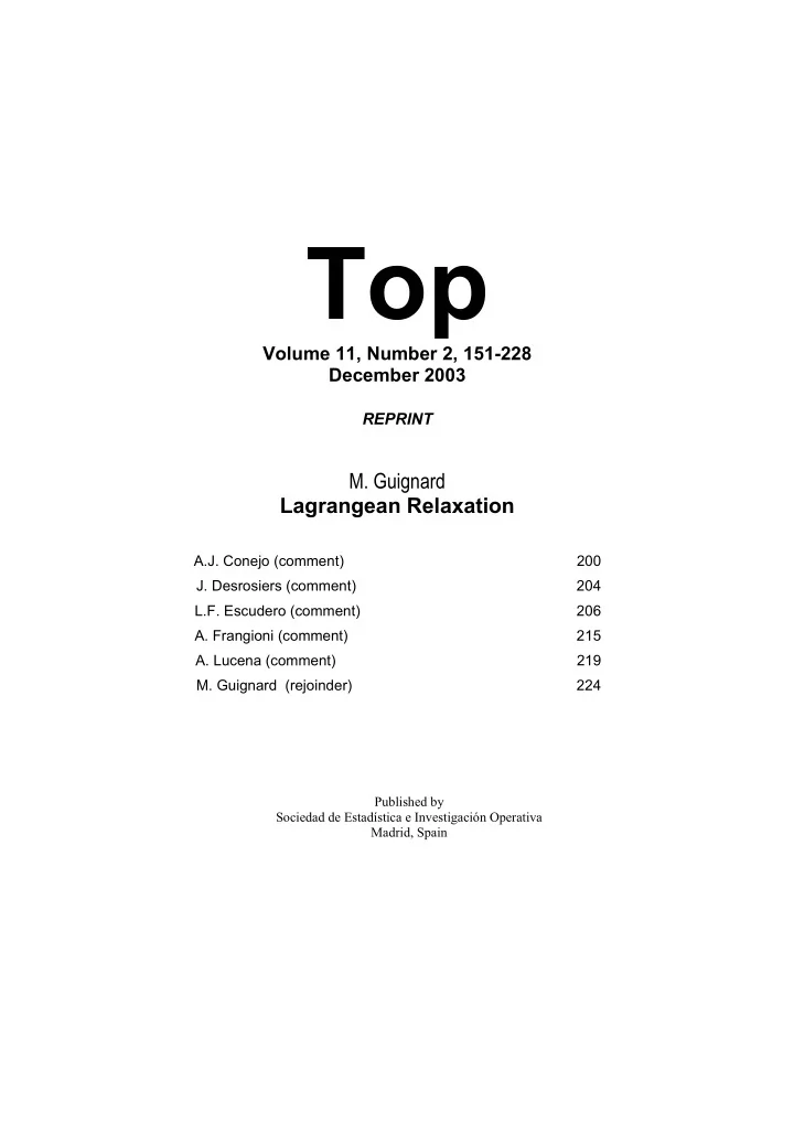
Figure 2

taken by a given yi decides alone the fate of all other variables containing the same value of the index i – that usually means that if variable yi is 0, all variables in “its family” are 0, and if it is 1, they are solutions of a subproblem – one may be able to reformulate the problem in terms of the variables yi only. Often, but not always, when this property holds, it is because the Lagrangean problem, after removal of all constraints containing

nly the yi’s – let us call it (LRPλ), for partial problem – decomposes into
ne problem (LRP i

λ) for each i, i.e., for each 0-1 variable yi.

The use of this property is based on the following fact. In problem (LRP i

λ), the integer variable yi can be viewed as a parameter, however we

do know that for the mixed-integer problem (LRP i

λ), the feasible values of

that parameter are only 0 and 1, and we can make use of the fact that there are only two possible values for v(LRP i

λ), the value computed for yi = 1,

say vi (= vi · yi for yi = 1), and the value for yi = 0, that is, 0 (= vi · yi for yi = 0), which implies that for all possible values of yi, v(LRP i

λ) = vi · yi.

Hence the name “integer linearization”, as one replaces a piecewise linear function corresponding to 0 ≤ yi ≤ 1 by a line through the points (0, 0) and (1, vi). We will first present an example of the simple decomposable case. Example 6.1. Suppose that (LRλ) is of the form minx{fx + gy | Aixi ≤ piyi, all i, x ∈ X, By ≤ b, yi = 0 or 1, all i}, where there is one set of constraints Aixi ≤ piyi for each i, the constraints By ≤ b are over y alone, Ai and pi are nonnegative, and X = Πi(Xi). Here xi may be a vector, with possibly some integer part. To solve (LRλ), one can proceed as follows: (i) ignore at first the constraints containing only the yi’s, i.e., By ≤ b;

SLIDE 15

Lagrangean Relaxation

163 (ii) given the model, it is clear that the problem then separates into one problem for each i: min{fixi + giyi | Aixi ≤ piyi, xi ∈ Xi, yi = 0 or 1} (LRi

λ)

where yi plays the role of a 0-1 parameter: for yi = 0, xi = 0, and fixi + giyi = 0, for yi = 1, solve (LRi

λ | yi = 1): let vi = min{fixi + gi | Aixi ≤

pi, xi ∈ Xi}, then vi is the contribution of yi = 1 in the objective function. (iii) replace v(LRλ) by v(PLλ) where problem (PLλ), usually much simpler to solve than (LRλ), is min{

viyi | By ≤ b, yi = 0 or 1, all i}. (PLλ) This process makes use of the integrality constraint on variable yi and therefore even in cases where both (PLλ) and (LRi

λ | yi = 1) have the

Integrality Property, it is possible to have v(LR) = min

λ v(PLλ) = min λ v(LRλ) < v(LP).

Example 6.2. We will now present a somewhat more complicated example

f ILP than the above model. de Matta and Guignard (1994) presents a

production scheduling problem for a tile manufacturing company. There are several aggregate families of tiles, indexed by I, and i ∈ I stands for a type of tiles that share important characteristics (size, color, material, required oven temperature,. . . ). If it is allowed to leave a machine idle, we will say that it is producing product i = 0 (that is, the “idle product”). The bottleneck in the production line is tile baking, which is done in kilns, j ∈ J. The kiln temperature must remain constant through the baking process. Each kiln j bakes tiles of a certain type i at a certain temperature, and therefore at a certain (constant) weekly production rate pij (related to the flow rate of the cars loaded with tiles as they enter the kilns). Changeover takes place only between weeks, and there is a changeover cost rlij as well as a production loss Klij on machine (kiln) j for changing from product (tile type) l to product i. In the original problem, backlogging was not allowed, but we will consider here the more general case where the demand

SLIDE 16

164

M. Guignard

dis for tile type i in week s can be met by producing it in any period t during the time horizon, i.e.,t ∈ {1, 2, . . . , T}. We will use T + 1 as the name of the first period (week) beyond the time horizon. The reason we need to consider it is that the production rate being fixed, we may end up with remaining inventories in period T + 1. For consistency we also define di,T+1 = max(

s dis, j pij).

We are using a disaggregated model (similar in spirit to that of Bowman (1956)) which yields a tight LP relaxation bound, and provides interesting structural characteristics. Let xijts be the percentage of the demand dis produced on machine j in period t, and let ylijt be a 0-1 variable equal to 1 if there is a production changeover from l to i on machine j at the beginning

f period t, 0 otherwise. One knows which product lj each machine j was

producing in the week preceding the first week (initial conditions). Let cijts be the cost of either holding or backlogging the demand dis between periods t and s if produced on j. The model can then be stated as follows: min

i,j,t,s

cijtsxijts +

l,i,j,t

rlijylijt +

i,j,t

cijt,T+1xijt,T+1 (IP) s.t.

xijts ≥ 1 ∀i, s

disxijts =

(pij − Klij)ylijt ∀i, j, t

yljij1 = 1 ∀j

ylijt =

yikj,t+1 ∀i, j, t

ylijT = 1 ∀j xijts ≥ 0, ylijt ∈ {0, 1}, ∀l, i, j, t, s If we dualize the demand constraint (the first constraint) with nonnegative multiplier λ, the Lagrangean relaxation (LRλ) reads min

i,j,t,s

cijtsxijts +

l,i,j,t

rlijylijt +

i,j,t

cijt,T+1xijt,T+1+ +

λis(1 −

xijts) (LRλ)

SLIDE 17

Lagrangean Relaxation

165 s.t.

disxijts =

(pij − Klij)ylijt ∀i, j, t

yljij1 = 1 ∀j

ylijt =

yikj,t+1 ∀i, j, t

ylijT = 1 ∀j xijts ≥ 0, ylijt ∈ {0, 1}, ∀l, i, j, t, s The first remark is that the model decomposes into one problem for each machine j. Let (LRj

λ) be the subproblem corresponding to machine j:

min

i,t,s

(cijts − λls)xijts +

l,i,t

rlijylijt +

cijt,T+1xijt,T+1 (LRj

λ)

s.t.

disxijts =

(pij − Klij)ylijt ∀i, t

yljij1 = 1

ylijt =

yikj,t+1 ∀i, t

ylijT = 1 xijts ≥ 0, ylijt ∈ {0, 1}, ∀l, i, t, s In the first constraint of (LRj

λ), the right hand side contains not one, but a

set of 0-1 variables, so the structure is different from that presented above. However, the second and third constraint together imply that exactly one ylijt is equal to 1, for every i and t. That is, including if necessary the “idle product”, at the beginning of period t, machine j switches to exactly

ne product i from exactly one product l (which may actually be i = l).

Therefore if ylijt = 1,

ykijt = 0 and one can find the corresponding xijts and xijt,T+1 by solving the continuous knapsack-like problem min

(cijts − λls)xijts + cijt,T+1xijt,T+1 (P l,i,j,t

) s.t.

disxijts = pij − Klij

SLIDE 18

166

M. Guignard

0 ≤ xijts ≤ 1, xijt,T+1 ≥ 0. (LRj

λ) then reduces to

min

l,i,t

(v(P l,i,j,t

) + rlij)ylijt s.t.

yljij1 = 1

yljijt =

yikj,t+1 ∀i, t

ylijT = 1 ylijt ∈ {0, 1} ∀l, i, t This problem can be solved as an acyclic shortest path problem, which amounts to searching for a sequence of changes for machine j, from period to period, from a product to another (or maybe the same) product. A node corresponds to setting up machine j in period t to produce product

i. An arc from node (i, j, t − 1) to node (l, j, t) has cost v(P i,i,j,t

) if i = l (one continues to produce i in period t), and it is associated with yiijt = 1,

r it has cost v(P i,l,j,t

) + rilj if i = l (one switches from i to l), and it is associated with yiljt = 1. Notice that arc costs may be negative. To summarize, the Lagrangean problem decomposes into one problem per machine j, and these problems for machine j can be solved by solving

ne continuous knapsack-like problem per (l, i, t) (i.e., per arc), and one

shortest path problem. Notice however that the Lagrangean problem does not have the integrality property. An example given in de Matta (1989) proves this fact. One may (and actually does) obtain LR bounds much tighter than the LP bound, even though the subproblems are trivial to solve.

7 Constructing a Lagrangean Relaxation

There are often many ways in which a given problem can be relaxed in a Lagrangean fashion. We will list here a few, mostly to point out that often some reformulation prior to relaxation can help, and that for many complex

SLIDE 19

Lagrangean Relaxation

167 models, intuition and some understanding of the constraint interactions may suggest ingenious and efficient relaxation schemes. (1) One can isolate an interesting subproblem and dualize the

ther constraints.

This is the most commonly used approach. It has the advantage that the Lagrangean subproblems are “interesting” (in the sense usually that they have a special structure that can be exploited) and there may even exist specialized algorithms for solving them efficiently. (2) If there are two (or more) interesting subproblems with common variables, one can split these variables first, then dualize the copy constraint. This is called Lagrangean decomposition (LD) (Soenen (1977)), variable splitting (N¨ asberg et al. (1985)) or variable layering, Glover and Kling- mann (1988). Shepardson and Marsten (1980), and Ribeiro and Minoux (1986) are among the early papers introducing the approach. One must first reformulate the problem using variable splitting, in other words, one must rename the variables in part of the constraints as if they were independent variables. Problem (P) : minx{fx | Ax ≤ b, Cx ≤ d, x ∈ X} is clearly equivalent to problem (P ′) : minx,y{fx | Ax ≤ b, x ∈ X, Cy ≤ d, y ∈ X, x = y}, in the sense that they have equal optimal values (but notice that they have different variable spaces). In addition if x∗ is an optimal solution of (P), then the solution (x, y) ≡ (x∗, x∗) is optimal for (P ′), and if (x∗, y∗) is an optimal solution of (P ′), then x∗ = y∗ and x∗ is optimal for (P). One dualizes the copy constraint x = y in (P ′) with multipliers λ, this separates the problem into an x-problem and a y-problem: min

x,y {fx + λ(y − x) | Ax ≤ b, x ∈ X, Cy ≤ d, y ∈ X}

(LDλ) = min

x {(f − λ)x | Ax ≤ b, x ∈ X} + min y {λy | Cy ≤ d, y ∈ X}.

This process creates a staircase structure, and thus decomposability, in the

model. Notice that here λ is not required to be nonnegative.

Remember also that when one dualizes equality constraints, a feasible Lagrangean solution is automatically optimal for the original integer pro-

SLIDE 20

168

M. Guignard

Co{xXCxd}

{xCxd}

{xAx b} V(LR) Co{xXAxb}

V(LD) x x x x x x x x x x x x

Figure 3: Geometric interpretation of Lagrangean decomposition

gramming problem. The copy constraint being an equality constraint, if both Lagrangean subproblems have the same optimal solution, that solution is optimal for the IP problem. Guignard and Kim (1987) showed that the LD bound can strictly dom- inate the LR bounds obtained by dualizing either set of constraints: Theorem 7.1. If v(LD) = maxλ[minx{(f − λ)x | Ax ≤ b, x ∈ X} + miny{λy | Cy ≤ d, y ∈ X}] then v(LD) = min

fx | x ∈ Co{x ∈ X | Ax ≤

b} ∩ Co{x ∈ X | Cx ≤ d}

This geometric interpretation is demonstrated in Figure 3. Corollary 7.1.

If one of the subproblems has the Integrality Property, then v(LD) is

equal to the better of the two LR bounds corresponding to dualizing either Ax ≤ b or Cx ≤ d.

If both subproblems have the Integrality Property, then v(LD) = v(LP).

If one applies LD to the GAP by splitting the constraints into two nonoverlapping subsets, the (KP) and the (MC) constraints, one then

btains the same bound as when dualizing the multiple choice constraints.

SLIDE 21

Lagrangean Relaxation

169 It would then seem to be uninteresting to split the variables, as this requires a number of multipliers equal to the number of machines times the number

f jobs, as compared to only the number of jobs with the strong Lagrangean
relaxation. It is possible though that Lagrangean solutions can exploit the

two Lagrangean solutions obtained and it might be worth the extra work of solving the Lagrangean decomposition dual, J¨

rnsten and N¨

asberg (1986). Occasionally the variable splitting will correspond to a physical split of

ne of the problem’s decision variables. This is illustrated by the following

example. Example 7.1. Guignard and Yan (1993), and Yan (1996) describe the following problem and scheme for a hydroelectric power management problem. Electric utility production planning is the selection of power generation and energy efficiency resources to meet customer demands for electricity

ver a multi-period time horizon. The project described in the paper is

a real-world hydropower plant operations management problem of a dis- patch type. The system consists of a chain of 10 consecutive hydropower plants separated by reservoirs and falls with 23 identical machines installed to generate electric power. Specifically there are two machines installed in eight power plants (plants 1, 2, 3, 4, 5, 6, 7, and 10), three machines in

ne power plant (plant 8) and four machines in the last power plant (plant

9). Each machine has two or four work parts for producing electric power, according to different water throughput. Since demand for electric power varies with different time periods, power plant managers must make optimal decisions concerning the number of machines that should be operated in each power plant during each time period. Managing the power generation requires decisions concerning water releases at each plant k in each time period. A period is two hours. The model (which is confidential) was constructed by an independent consulting firm. This results in a large complex mixed-integer program. The problem is complex, with 2691 variables, 384 of which are binary, and 12,073 constraints. The firm had tried to solve the problem for the utility company with several of the best MIP software packages available, with help from the software companies themselves. Yet they did not succeed. Guignard and Yan repeated the tests with several solvers running under GAMS, on several RISC systems, also to no avail. The best result after 5 days and six hours on an HP workstation was a bracket [3174.97, 3534.17], i.e., a residual gap of more than 11%.

SLIDE 22

170

M. Guignard

Power Plant k Power Plant k+1 low water level of k high water level of k+1

Figure 4: Variable splitting

In order to reduce the complexity of the model, they tried several La- grangean relaxations and decompositions. One of the decompositions tested consists in “cutting” each reservoir in half (see Figure 4), i.e. “splitting” the water level variable in each reservoir, and dualizing the following copy constraint: high water level in k + 1 = low water level in k. This Lagrangean decomposition produces one power management problem per power plant k. These subproblems do not have a special structure, but are much simpler and smaller than the original problem, are readily solvable by commercial software, and do not have the Integrality Property. They were solved by Branch-and-Bound. This LD shrinks problem size, and yields Lagrangean bounds much stronger than the LP bounds. In addition the Lagrangean solutions can be modified to provide feasible schedules.

SLIDE 23

Lagrangean Relaxation

171 (3) One can dualize linking constraints. Sometimes naturally, sometimes after some reformulation, problems may contain independent structures linked by some constraints: minx,y{fx + gy | Ax ≤ b, x ∈ X, Cy ≤ d, y ∈ Y, Ex + Fy ≤ h}. Dualizing the linking constraints Ex + Fy ≤ h splits the problem into an x-problem and a y-problem. Sometimes the original problem only contains x and some reformulation introduces a new variable y, while the relationship between x and y is captured by the new constraints Ex + Fy ≤ h. Example 7.2. A production problem over multiple facilities contains constraints related to individual facilities, and the demand constraints link all plant productions. If one dualizes the demand constraints, the Lagrangean problem decomposes into a production problem for each facility, which is typically much easier to solve than the overall problem. If at least one

f these subproblems does not have the Integrality Property, this LR may

yield a tighter bound than the LP bound. In Andalaft et al. (2003), a forest company must harvest geographically distinct areas, and dualizing the demand constraints splits the problem into one subproblem per area, which is typically much easier to solve than the overall problem. Example 7.3. Consider a multi-period model in which facilities built in

ne period can be used in that or a later period. One may be able to use

“action” (building) variables (say, binary variable xit, equal to 1 iff one builds facility i in period t) in the “design” part of the model, and “state” (existence) variables (say, binary variable yit, equal to 1 iff facility i exists in period t) in the rest of the model. Thus yit ≥ yi,t−1 for all i and t. The relationship between the two sets of variables is captured by the following constraints: xit ≥ yit − yi,t−1 and yit ≥ xiτ, ∀i, t, and τ ≤ t. Both types of constraints are necessary to enforce that xit is 1 only in the building period, i.e., when yit is 1 and yi,t−1 is 0, and yiτ remains 0 until the smallest period τ = t for which xit is 1. Dualizing these linking relationships between “built in period t” and “built by period t” may split the model into a facility-building problem and a facility-using problem. If neither has the Integrality Property, the Lagrangean relaxation bound can be stronger than the LP bound. See for instance Chajakis et al. (1994).

SLIDE 24

172

M. Guignard

This is actually a special case of Lagrangean substitution (LS), where Ex + Fy ≤ h is the copy constraint introduced in the reformulation. (4) One can sometimes dualize aggregate rather than individual copies of variables. Instead of creating a copy y of variable x and introducing y into model (P) by rewriting the constraint Cx ≤ d as Cy ≤ d, to yield the equivalent model (P ′): minx,y{fx | Ax ≤ b, x ∈ X, Cy ≤ d, y ∈ X, x = y}, one can also create a problem (P ′′) equivalent to problem (P) by introducing a new variable y and forcing the constraint Dy = Cx. This constraint is in general weaker than the constraint x = y. Model (P ′′) is minx,y{fx | Ax ≤ b, x ∈ X, Dy ≤ d, y ∈ X, Dx = Cy}. The LR introduced here dualizes the aggregate copy constraint Dx = Cy. Here again the copy constraint is an equality constraint, therefore if the Lagrangean subproblems have optimal solutions x and y that satisfy the aggregate copy constraint, i.e., if Dy = Cx, then the x-solution is optimal for the IP problem. Example 7.4. Consider the bi-knapsack problem max

x {

cixi |

bixi ≤ m,

dixi ≤ n, xi ∈ {0, 1}, ∀i}. (BKP) One can introduce a new variable y, and write

i bixi = i biyi. The

equivalent problem is max

x,y {

cixi |

biyi ≤ m,

dixi ≤ n,

bixi =

biyi, xi, yi ∈ {0, 1}, ∀i} (BKP′) and the LR problem is max

x,y {

cixi − λ(

bixi −

biyi) |

biyi ≤ m,

dixi ≤ n, xi, yi ∈ {0, 1}, ∀i} (LRλ) = max

x {

(ci − λbi)xi |

dixi ≤ n, xi ∈ {0, 1}, ∀i} + max

y {λ

biyi) |

biyi ≤ m, yi ∈ {0, 1}, ∀i}.

SLIDE 25

Lagrangean Relaxation

173 Here λ is a single real multiplier of arbitrary sign. The Lagrangean bound produced by this scheme is in between that of the LP bound and that of the Lagrangean decomposition bound obtained by dualizing xi = yi ∀i. This is similar in spirit to the copy constraints introduced in Reinoso and Maculan (1988). It would seem natural that a reduction in the number of multipliers should imply a reduction in the quality of the LR bound obtained. This is not always the case, however, as shown in example 7.5. Example 7.5. Chen and Guignard (1998) consider an aggregate Lagrangean relaxation of the capacitated facility location problem. The model uses continuous variables xij that represent the percentage of the demand dj

f customer j supplied by facility i, and binary variables yi, equal to 1 if

facility i with capacity ai is operational. The constraint

djxij ≤ aiyi imposes a conditional capacity restriction on the total amount that can be shipped from potential facility i. min

x,y

cijxij +

fiyi (CPLP) s.t.

xij = 1, all j

meet 100% of customer demand

(D) xij ≤ yi, all i, j

ship nothing if plant is closed

(B)

aiyi ≥

dj, all j

enough plants to meet total demand

(T)

djxij ≤ aiyi, all i

ship no more than plant capacity

(C) xij ≥ 0, yi = 0 or 1, all i, j. Constraint (T) is redundant, but may help getting tighter Lagrangean relaxation bounds. The three best Lagrangean schemes are: (LR) Geoffrion and McBride (1978), Ryu and Guignard (1992). One dualizes (D) then uses the integer linearization property. The subproblems to solve are one continuous knapsack problem per plant

SLIDE 26

174

M. Guignard

and one 0-1 knapsack problem over all plants. The Lagrangean relaxation bound is tight, and it is obtained at a small computational cost. (LD) Guignard and Kim (1987). Duplicate (T). Make copies xij = x′

ij and yi = y′ i and use x′ ij and y′ i

in (C) and in one of the (T). One obtains the split {(D), (B), (T)} → APLP (see Thizy (1994), Ryu (1992) for solutions methods for APLP) {(B), (T), (C)} → this is like in (LR) This LD bound is tighter than the (LR) bound, but expensive to compute, in particular because of a large number of multipliers. (LS) Chen and Guignard (1998). Copy

j djxij = j djx′ ij and yi = y′ i in (C). This yields the same

split as (LD), and the same bound, as proved in Chen and Guignard (1998). This is very surprising, as it is less expensive to solve (LS) than (LD), in particular because (LS) has far fewer multipliers. In example 7.5, creating new copy variables x′

ij and y′ i, one can create

an LS by dualizing the aggregate (linking) copy constraints

djxij =

djx′

ij and aiyi = aiy′ i . Surprisingly (see Chen and Guignard (1998)

for details), one can prove that the LS bound for this problem is as strong as the LD bound obtained by dualizing individual copies xij = x′

ij and

yi = y′

i. This suggests that “aggregating” variables before copying them

may be an attractive alternative to Lagrangean decomposition, at least for some problem structures. A more general structure than CPLP is actually described in Chen and Guignard (1998).

8 Characteristics of the Lagrangean Function

The Lagrangean function z(λ) = v(LRλ) is an implicit function of λ. Sup- pose that the set Co{x ∈ X | Cx ≤ d} is a polytope, i.e., a bounded polyhedron, then there exists a finite family {x1, x2, . . . , xK} of extreme points

SLIDE 27

Lagrangean Relaxation

175

= f x2 + (b-A x2)

= f x1 + (b-A x1)

f x1 f x2 = f xk + (b-A xk) f xk

Figure 5: The Lagrangean function for the maximization case

f Co{x ∈ X | Cx ≤ d}, i.e., of points of {x ∈ X | Cx ≤ d}, such that

Co{x ∈ X | Cx ≤ d} = Co{x1, x2, . . . , xK}. It then follows that min

x {fx + λ(Ax − b) | Cx ≤ d, x ∈ X} =

min

k=1,...,K{fxk + λ(Axk − b)}

and z(λ) is the lower envelope of a family of linear functions of λ , fxk + λ(Axk − b), k = 1, . . . , K, and thus is a concave function of λ , with break- points where it is not differentiable, i.e., where the optimal solution of (LRλ) is not unique. Figure 5 shows a Lagrangean function for the case where (P) is a maximization problem, this (LR) is a minimization problem, and z(λ) a convex function of (λ). A concave function f(x) is continuous over the relative interior of its domain, and it is differentiable almost everywhere, i.e., except over a set of measure 0. At points where it is not differentiable, the function does not have a gradient, but it always has subgradients. Definition 8.1. A vector y ∈ (Rn)∗ is a subgradient of a concave function

SLIDE 28

176

M. Guignard

f(x) at a point x0 ∈ Rn if for all x ∈ Rn f(x) − f(x0) ≤ y · (x − x0). Definition 8.2. The set of all subgradients of a concave functionf(x) at a point x0 is called the subdifferential of f at x0 and it is denoted ∂f(x0). Theorem 8.1. The subdifferential ∂f(x0) of a concave function f(x) at a point x0 is always nonempty, closed, convex and bounded. If the subdifferential of f at x0 consists of a single element, that element is the gradient of f at x0, denoted by ∇f(x0). The dual problem (LR) is max

λ≥0 v(LRλ) = max λ≥0 z(λ)

(LR) = max

λ≥0

min

k=1,...,K{fxk + λ(Axk − b)}

= max

λ≥0,η{η | η ≤ fxk + λ(Axk − b), k = 1, . . . , K}.

Let λ∗ be a minimizer of z(λ), and let η∗ = z(λ∗). Let λk be a current “guess” at λ∗, let ηk = z(λk), and let Hk = {λ | fxk + λ(Axk − b) = ηk} be a level hyperplane passing through λk.

If z(λ) is differentiable at λk, i.e., if (LRλ) has a unique optimal

solution xk, it has a gradient ∇z(λk) at λk: ∇T z(λk) = (Axk − b) ⊥ Hk.

If z(λ) is nondifferentiable at λk, i.e., if (LRk

λ) has multiple opti-

mal solutions, one can show that the vector sk = (Axk − b)T is a subgradient of z(λ) at λk. That vector sk is orthogonal to Hk. If one considers the contours C(α) = {λ ∈ Rm

+ | z(λ) ≥ α}, α a scalar, these

contours are convex polyhedral sets. See Figure 6. A subgradient is not necessarily a direction of increase for the function, even locally, as seen on Figure 6.

SLIDE 29

Lagrangean Relaxation

177

* k Hk = {f xk + ( Axk -b) = k} region where xk is optimal for (LR ) sk = (Axk- b)T C(=k) Space of Figure 6: Contours of the Lagrangean function

9 Primal and Dual Methods to Solve Relaxation Duals

A number of methods have been proposed to solve Lagrangean duals. They are either ad-hoc, like for instance dual ascent methods, or general purpose, usually aiming at solving a generic nonsmooth convex optimization prob-

lem. This section reviews the most important approaches.

9.1 Subgradient Method This method was proposed in Held and Karp (1971), then validated in Held et al. (1974). See also Poljak (1977). It is an iterative method in which at iteration k, given the current multiplier vector λk, a step is taken along a subgradient of z(λk), then, if necessary, the resulting point is projected

nto the nonnegative orthant.

SLIDE 30

178

M. Guignard

Let x(k) be an optimal solution of (LRk

λ). Then sk = (Ax(k) − b)T is a

subgradient of z(λ) at λk. If λ∗ is an (unknown) optimal solution of (LR), with η∗ = z(λ∗), let λ′k+1 be the projection of λk on the hyperplane H∗ parallel to Hk, defined by H∗ = {λ | fxk + λ(Ax(k) − b) = η∗}. The vector sk is perpendicular to both Hk and H∗, therefore λ′k+1 − λk is a nonnegative multiple of sk: λ′k+1 − λk = µsk, µ ≥ 0. Also, λ′k+1 belongs to H∗: fx(k) + λ′k+1(Ax(k) − b) = η∗ therefore fxk + λk(Axk − b) + µsk(Ax(k) − b) = ηk + µsk · sk = η∗ and µ = η∗ − ηk sk2 , so that λ′k+1 = λk + sk(η∗ − ηk) sk2 . Finally define λk+1 = [λ′k+1]+, i.e., define the next iterate λk+1 as the projection of λ′k+1 onto the nonnegative orthant, as λ must be nonnegative. Given the geometric projections described above, it is clear that λk+1 is closer to λ∗ than λk, thus the sequence λk −λ∗2 is monotone nonincreas- ing. Remark 9.1. This formula unfortunately uses the unknown optimal value η∗ of (LR). One can try to use an estimate for that value, but then one may be using either too small or too large a multiple of sk. If one sees that the objective function values do not improve for too many iterations,

ne should suspect that η∗ has been overestimated (for a maximization

problem) and that one is “overshooting”, thus one should try to reduce the difference η∗ − ηk. This can be achieved by introducing from the start a positive factor ǫk ∈ (0, 2), in the subgradient formula: λk+1 = λk + sk · ǫk(η∗ − ηk) sk2 , and reducing the scalar ǫk when there is no improvement for too long.

SLIDE 31

Lagrangean Relaxation

179 Practical convergence of the subgradient method is unpredictable. For some problems, convergence is quick and fairly reliable, while other problems tend to produce erratic behavior of the multiplier sequence, or of the Lagrangean value, or both. In a “good” case, one will usually observe a saw- tooth pattern in the Lagrangean value for the first iterations, followed by a roughly monotonic improvement and asymptotic convergence to a value that is hopefully the optimal Lagrangean bound. In “bad” cases, the saw- tooth pattern continues, or, worse, the Lagrangean value keeps deteriorat-

ing. Many authors have studied this problem and have proposed remedies.

Camerini et al. (1975) and Bazaraa and Sherali (1981) are two often-quoted papers devoted to improving algorithmic behavior via improved computa- tions of the subgradient step size. 9.2 Dual ascent methods In this kind of approach, one takes advantage of the structure of the La- grangean dual to create a sequence of multipliers that guarantee a monotone increase in Lagrangean function value. This approach had been pioneered by Bilde and Krarup (1967) and Bilde and Krarup (1977) for solving approximately the LP relaxation of the uncapacitated facility location problem (UFLP). Erlenkotter (1978) independently developed a dual ascent method for solving a Lagrangean relaxation of the same uncapacitated location problem. This Lagrangean bound, because of the Integrality Prop- erty, was actually equal to the LP bound of Bilde and Krarup (1967). The LP size for UCLP gets very large for even moderate size problems, and both approaches were successful at producing optimal LP values in a large proportion of all cases tried. In addition the primal solutions found by Er- lenkotter (1978) were often optimal for the UFLP as a very large percentage

f the LP solutions are actually integer.

In general though one cannot expect that LP solutions will almost always be integer, and dual ascent methods normally concentrate on the dual task of optimizing the Lagrangean dual problem. These approaches are structure-dependent and thus problem specific. Some examples of successful Lagrangean dual ascent design and implementation are Fisher and Hochbaum (1980), Fisher et al. (1986), Fisher and Kedia (1990) and Guig- nard and Rosenwein (1990). General principles for developing a successful Lagrangean dual ascent method can be found in Guignard and Rosenwein (1989).

SLIDE 32

180

M. Guignard

9.3 Constraint Generation Method (also called cutting plane method, or CP) In this method Cheney and Goldstein (1959) and Kelley (1960), one uses the fact that z(λ) is the lower envelope of a family of linear functions: max

λ≥0 v(LRλ) = max λ≥0 z(λ)

(LR) = max

λ≥0

min

k=1,...,K{fxk + λ(Axk − b)}

= max

λ≥0,η{η | η ≤ fxk + λ(Axk − b), k = 1, . . . , K}.

At each iteration k, one generates one or more cuts of the form η ≤ fxk + λ(Ax(k) − b), by solving the Lagrangean subproblem (LRk

λ) with solution x(k). These cuts

are added to those generated in previous iterations to form the current LP master problem: max

λ≥0,η{η | η ≤ fx(h) + λ(Ax(h) − b), h = 1, . . . , k},

(MP k) whose solution is the next iterate λk+1. The process terminates when v(MP k) = z(λk+1). This value is the optimal value of (LR). 9.4 Column generation (CG) (CG) has been used extensively, in particular for solving very large scheduling problems (airline, buses, . . . ). It consists in reformulating a problem as an LP (or an IP) whose activities (or columns) correspond to feasible solutions of a subset of the problem constraints, subject to the remaining

constraints. The variables are weights attached to these solutions.

There are two aspects to column generation: first, the process is dual to Lagrangean relaxation and to CP. Secondly, it can be viewed as an application of Dantzig and Wolfe’s decomposition algorithm, Dantzig and Wolfe (1960) and Dantzig and Wolfe (1961). Let the xk ∈ {x ∈ X | Cxk ≤ d}, k ∈ K, be chosen such that Co{xk} = Co{x ∈ X | Cx ≤ d}. A possible choice for the xk’s is all the points of Co{x ∈ X | Cx ≤ d} but a cheaper

ption is all extreme points of Co{x ∈ X | Cx ≤ d}.

SLIDE 33

Lagrangean Relaxation

181 Problem (P) : minx{fx | Ax ≤ b, Cx ≤ d, x ∈ X} yields the Lagrangean dual (i.e., in the λ -space) problem max

λ≥0 min x {fx + λ(Ax − b) | Cx ≤ d, x ∈ X}

(LR) which is equivalent to the primal (i.e., in the x-space) problem min

fx | Ax ≤ b, x ∈ Co{x ∈ X | Cx ≤ d}
,

(PR) which itself can be rewritten as min

f(
k∈K

µkxk) | A(

k∈K

µkxk)x ≤ b,

k∈K

µk = 1, µk ≥ 0

(PR)

= min

k∈K

µk · (fxk) |

k∈K

µk · (Axk) ≤ b,

k∈K

µk = 1, µk ≥ 0

given that one can write x ∈ Co{x ∈ X | Cx ≤ d} as x =

k∈K

µkxk, with

k∈K

µk = 1 and µk ≥ 0. The separation of a problem into a master- and a sub-problem is equivalent to the separation of the constraints into kept and dualized constraints. The columns generated are solutions of integer subproblems that have the same constraints as the Lagrangean subproblems. Column generation was used for instance in Savelsbergh (1997) for the strong Lagrangean relaxation of the GAP. The bounds obtained were usually very tight, i.e., much closer to the true IP value than the LP bound. The value of the LP relaxation of the master problem is equal to the Lagrangean relaxation bound. The strength of a CG or LR scheme would then seem to be based on the fact that the subproblems do not have the integrality property. It may happen however that such a scheme can be successful at solving problems with the integrality property because it permits the indirect computation of v(LP) when this value could not be computed directly, e.g., because of an exponential number of constraints, Held and Karp (1970), Held and Karp (1971). One substantial advantage of (CP) or (CG) over subgradient algorithms is the existence of a true termination criterion v(MP k) = z(λk+1). Although for certain families of problems, such as some multi-item capacitated lot-sizing problems with or without setup times, Guignard et al.

SLIDE 34

182

M. Guignard

(2002), (CG) can converge very quickly (in no more than fifteen to twenty iterations in that lot-sizing application), it often happens in practice that the process of generating enough constraints (in CP) or enough columns (in CG) to achieve convergence takes a very long time. First in the initial steps only a few constraints/columns are known and the approximation of the Lagrangean function may be quite poor. It may take a while until the family of constraints/columns generated permits a relatively accurate localization of the optimal multiplier vector. Secondly towards the end of the process it often happens that the problems are highly degenerate, and many iterations may be performed without true improvement either in multiplier

r in Lagrangean value. Many attempts have been made to correct this
behavior. Going into greater details is beyond the scope of this paper, we

will just mention a few possible approaches, described in du Merle et al. (1998), du Merle et al. (1999), and Wentges (1997). 9.5 Bundle methods Lemar´ echal (1974) and Zowe (1985) introduced an extension of subgradient methods, called bundle methods, in which past information is collected to provide a better approximation of the Lagrangean function. The standard CP algorithm uses the bundle of the subgradients that were already generated, and constructs a piecewise linear approximation of the Lagrangean

function. This method is usually slow and unstable. Three different stabi-

lization approaches have been proposed. At any moment, one has a model representing the Lagrangean function, and a so-called stability center, which should be a reasonable approximation of the true optimal solution. One generates a next iterate which is a compromise between improving the objective function and keeping close to the stability center. The next iterate becomes the new stability center (a serious step) only if the objective function improvement is “good enough”. Otherwise, one has a null step, in which however one improves the function approximation. In addition, this “next iterate” shouldn’t be too far away from the “stability center”. The three stabilization approaches propose different ways of controlling the amount of move that is allowed. Either the next iterate must remain within a so-called trust region, or one adds a penalty term to the approximation of the function that increases with the distance from the stability center, or

ne remains within a region where the approximation of the function stays

above a certain level (for a maximization problem). This proximity measure

SLIDE 35

Lagrangean Relaxation

183 is the one parameter that may be delicate to adjust in practical implemen-

tations. There is a trade-off between the safety net provided by this small

move concept, and the possibly small size of the bound improvement. 9.6 The volume algorithm (VA) The volume algorithm, Barahona and Anbil (2000), an extension of the subgradient algorithm, can be seen as a fast way to approximate Dantzig- Wolfe decomposition, with a better stopping criterion, and it produces primal as well as dual vectors by estimating the volume below the faces that are active at an optimal dual solution. It has been used successfully to solve large-scale LP’s arising in combinatorial optimization, such as set partitioning or location problems. In a way similar to the serious/null steps philosophy of bundle methods, Bahiense et al. (2002) defines green, yellow

r red steps for VA, and introduces a precise measure for the improvement

needed to declare a green (or serious) step. This addition yields a revised formulation (RVA) that is somewhere between VA and a specific bundle

method. The authors applied both VA and their modified algorithms to

Rectilinear Steiner problems. 9.7 Augmented Lagrangean methods Augmented Lagrangeans have been used mostly in nonlinear continuous programming and in stochastic optimization. They can however also be used in nonlinear integer programming (NLIP) - and as a consequence in linear integer programming as well - to solve directly primal relaxation problems, instead of solving problems in the dual space. Such an approach for the linear case can be found in Desrosiers et al. (1988). A primal relaxation for NLIP was introduced in Guignard (1994). It is equivalent to the Lagrangean relaxation in the linear case (see Theorem 5.1), but usually not in the nonlinear one. The Primal Relaxation Problem of the nonlinear integer programming problem min

x {f(x) | g(x) = 0, x ∈ P ∩ X}

(IP) relative to the equality constraints g(x) = 0, with P a rational polyhedron and X a set containing the integrality restrictions on the variables, is the

SLIDE 36

184

M. Guignard

continuous nonlinear problem inf

f(x) | g(x) = 0, x ∈ Co{P ∩ X}
(PR)

If the function f(x) is convex and g(x) linear, (PR) is equivalent (see Rockafellar (1970)) to the Lagrangean dual problem max

inf

f(x) + λg(x) | x ∈ Co{P ∩ X}
.

(LR∗) On the other hand, (PR) is equivalent to the Proximal Augmented La- grangean problem inf

f(x)+(α/2ρ)|x−x∗|2+u∗·g(x)+ 1

2ρ|g(x)|2 | x ∈ Co{P ∩X}

, (PAL)

for any ρ > 0, sufficiently large, and any positive α, where x∗ is an optimal solution of the original problem (PR), and u∗ the associated optimal multiplier corresponding to the dualized constraints g(x) = 0. (PAL) can be solved by an adaptation of the proximal method of multipliers, which takes into account the implicit constraints x ∈ Co{P ∩ X}, Con- tesse and Guignard (1995). The Proximal Augmented Lagrangean function, L(x, w, u, α, ρ) = f(x) + (α/2ρ)|x − w|2 + u · g(x) + 1

2ρ|g(x)|2 depends

n the approximation u of u∗, the approximation w of x∗, the proximal

parameter α and the penalty parameter ρ. There are several advantages in using an augmented Lagrangean rather than a penalty method. First, there exists a finite value ρ of the penalty coefficient ρ such that for any ρ larger than or equal to ρ, problem (PAL) is equivalent to problem (PR). Second, the multipliers are updated via a closed-form, fixed-step gradient formula ui(k + 1) = ui(k) + ρ(Aix(k) − bi), that guarantees convergence to the optimal Kuhn-Tucker multiplier u∗

i ,

without any parameter adjustment or estimation, as would be the case in subgradient methods. Finally, in the linear case, convergence is achieved in a finite number of iterations (see for instance Bertsekas (1982)). The advantage of including the proximal term (α/2ρ)|x − x∗|2 , α > 0, is that if f(x) and g(x) are convex, L(x, w, u, α, ρ) is strictly convex in x and has a unique minimum over x for given w, u, α and ρ . (PAL) can be solved by a linearization method such as the method of Frank and Wolfe, or, preferably, simplicial decomposition, known for its improved convergence properties.

SLIDE 37

Lagrangean Relaxation

185 The advantage of using Co{P ∩ X} instead of P ∩ X is that problem (PAL) can be solved efficiently via a linearization method such as simplicial decomposition because its constraint set is polyhedral, while the problem minx

f(x) + (α/2ρ)|x − x∗|2 + u∗(Ax − b) + (1

2)ρ|Ax − b|2 | x ∈ P ∩ X

general cannot. Contesse et al. (2002) describes a successful implementation of the Aug- mented Lagrangean approach for solving capacitated facility location problems with a nonlinear objective function. 9.8 Two-Phase hybrid methods Guignard and Zhu (1994) presented a method that combines the subgradient method in a first phase, and constraint generation in a second phase. The multipliers are first adjusted according to the subgradient formula, and at the same time, constraints corresponding to all known solutions of the Lagrangean subproblems are added to the LP master problem. The value

f the LP master problem is taken as the current estimate of the optimum
f the Lagrangean dual. This estimate gets more and more accurate as

iterations go by, so there is no need for any adjustment of the stepsize: one keeps ǫk = 1 ∀k. The Lagrangean relaxation bound and the value of the master problem provide a bracket on the dual optimum, and this yields a convergence test, like for the pure constraint generation method. One must make sure that the process does not cycle. If constraints get repeated, the master problem cannot improve. After the same cut has been generated a given number of times (say, 5 times), one can switch to a pure constraint generation phase. A similar hybrid method has been advocated more recently by Guig- nard and Fr´ eville (2000), combining (CG) with the subgradient method. It is well known that it is difficult to generate a good set of columns at the beginning of the algorithm, the paper suggests using an initial phase that generates the “outside walls” of the Lagrangean function dome, to use a graphical explanation of the procedure. If one views the (concave) La- grangean function as a dome in R, where Rmcorresponds to the Lagrangean multipliers λ and R to the Lagrangean function, then in the initial phase,

ne will try to generate faces that together define a bounded polyhedron

containing the Lagrangean dome. In Figure 7, the three faces defined by the solid lines (they are “outside walls”, although not all of them) define a

SLIDE 38

186

M. Guignard

1 2 Z()

Figure 7

bounded polyhedron. The dotted lines define faces of the dome that may be discovered later in the algorithm. The initial phase uses a subgradient algorithm with large step size, purposely “overshooting” to discover

utside walls. Once the column generation master problem is feasible (or

equivalently once the cutting plane LP is feasible), or possibly some iterations later if one thinks there is some advantage in generating a few more faces, one switches to either constraint or column generation. From our experience with column generation for the GAP, the columns (i.e. faces) generated in the first phase contain more useful information than those generated by the standard “phase 1” method (i.e., if one starts with arti- ficial columns with a high cost), as evidenced by the fact that fewer new columns need to be generated for convergence.

10 Subproblem Decomposition

In many cases, the Lagrangean subproblem decomposes into smaller problems, and this means that the feasible region is actually the Cartesian product of several smaller regions. One clear advantage is the reduction in

SLIDE 39

Lagrangean Relaxation

187 computational complexity for the Lagrangean subproblems: it is generally much easier to solve 50 problems with 100 binary variables each, say, than a single problem with 5,000 (i.e., 50×100) binary variables. It also means that in column generation, the columns (i.e., the vectors that are feasible solutions of the kept constraints) decompose into smaller subcolumns, and each subcolumn is a convex combination of extreme points

f a small region. By assigning different sets of weights to these convex

combinations, one allows “mix-and-match” solutions, in other words, one may combine a subcolumn for the first subproblem that was generated at iteration 10, say, with a subcolumn for the second subproblem generated at iteration 7, etc. , to form a full size column. If one had not decomposed the problem ahead of time, one may have had to wait a long time for such a complete column to be generated. By duality, this means that in a cutting plane environment, one can also generate “sub-cut” for each subproblem, which amounts to first replacing η by z + λb in max

λ≥0,η{η | η ≤ fx(h) + λ(Ax(h) − b), h = 1, . . . , k}

(MP k) = max

λ≥0,z{z + λb | z ≤ (f + λA)x(h), h = 1, . . . , k},

and then z by a sum of scalars zl, with zl ≤ (fl + λAl)x(h)

, where l is the index of the Lagrangean subproblem, fl, Al, and x(h)

are the lth portions of the corresponding submatrices and vectors, and xh

l is a Lagrangean solution

f the lth subproblem found at iteration h, yielding the disaggregated master

problem max

λ≥0,zl

{

zl + λb | zl ≤ (f + λA)lxh

l , h = 1, . . . , k}.

(MPDk) Example 10.1. Consider again the GAP (for the minimization case, although it would work in exactly the same way with maximization). We have seen that its strong Lagrangean relaxation is min

cijxij +

λj(1 −

xij) (LRλ) s.t.

aijxij ≤ bi, ∀i ∈ I (KP)

SLIDE 40

188

M. Guignard

xij ∈ {0, 1}, ∀i ∈ I, j ∈ J = min

(cij − λj)xij +

λj |

aijxij ≤ bi, ∀i, xij ∈ {0, 1}, ∀i, j

λj +

(cij − λj)xij |

aijxij ≤ bi, ∀i, xij ∈ {0, 1}, ∀i, j

and (LR) is the maximum with respect to λ of v(LRλ).

Let EP(KP) = {xk | k ∈ K} be the set of all integer feasible solutions

f the constraints (KP), and let EP(KPi) = {xk

i· | k ∈ Ki} be the set of all

integer feasible solution of the ith knapsack, with K =

Ki. Then a feasible solution of (LRλ) can be described by xij =

k∈Ki

µi

kxk ij,

∀i, j. The Lagrangean dual is equivalent to the aggregate master problem AMP: max

λ,ζ {ζ | ζ ≤

cijxk

ij +

λj(1 −

ij), k ∈ K}

(AMP) = max

λ,z {z +

λj | z ≤

(cij − λj)xk

ij, ∀k ∈ K}

with the substitution ζ = z +

j λj.

If we had first written the column generation formulation for the La- grangean dual, we would naturally have de-coupled the solutions of the independent knapsack subproblems, using the independent sets Ki instead

f K, the column generation master problem would have been disaggre-

gated: max

λ,z

zi +

λj (DMP) s.t. zi ≤

(cij − λj)xk

ij,

∀i, ∀k ∈ Ki and its dual min

µ {

k∈Ki
I,j

cijxk

ijµ(i) k |

k∈Ki
i

ijµ(i) k , ∀j,

k∈Ki

µ(i)

k = 1, ∀i, µi k ≥ 0},

SLIDE 41

Lagrangean Relaxation

189 is clearly the Dantzig-Wolfe decomposition of the primal equivalent (PR) min

x {

cijxij |

xij = 1, xij ≥ 0} (PR)

f (LR).

11 Relax-and-Cut

One question that often arises in the context of Lagrangean relaxation is how to strengthen the Lagrangean relaxation bound. One possible answer is the addition of cuts that are currently violated by the Lagrangean solu-

tion. It is clear however that adding these to the Lagrangean problem will

change its structure and may make it much harder to solve. One possible way out is to dualize these cuts. Remember that dualizing does not mean discarding! The cuts will be added to the set of “complicating constraints”, and intuitively they will be useful only if the intersection NI (for “new intersection”) of the new relaxed polyhedron and of the convex hull of the integer solutions of the kept constraints is “smaller” than the intersection OI (for “old intersection”) of the old relaxed polyhedron and of the convex hull of the integer solutions of the kept constraints. This in turn is only possible if the new relaxed polyhedron is smaller than the old one, since the kept constraints are the same in both cases. This has the following

implications. Consider a cut that is violated by the current Lagrangean

solution: (1) if the cut is just a convex combination of the current constraints, dualized and/or kept, it cannot possibly reduce the intersection, since every point of the “old” intersection OI will also satisfy it; so in particular surrogate constraints of the dualized constraints cannot help. See Figure 8. (2) if the cut is a valid inequality for the Lagrangean problem, then every point in the convex hull of the integer points of the kept constraints satisfies it, because every integer feasible solution of the Lagrangean subproblem does; (3) it is thus necessary for the cut to use “integer” information from both the dualized and the kept constraints, and to remove part of the inter-

SLIDE 42

190

M. Guignard

x() OI= NI

Figure 8: A surrogate constraint of the dualized constraints cannot improve the LR bound if dualized (the convex hull of integer solutions does not change)

section. (Remember that the Lagrangean solution is an integer point

required to satisfy only the kept constraints). A Relax-and-Cut scheme could proceed as follows:

1. initialize the Lagrangean multiplier λ.
2. solve the current Lagrangean problem, let x(λ) be the Lagrangean solu-
tion. If the Lagrangean dual is not solved yet, update λ . Else end.
3. identify a cut that is violated by x(λ), and dualize it. Go back to 2.

The term “Relax-and-Cut” was first used by Escudero et al. (1994). In that paper, a partial description of the constraint set was used, and violated constraints (not cuts) were identified, added to the model and immediately

dualized. The idea, if not the name, had actually been used earlier. For

instance in solving TSP problems, subtour elimination constraints were generated on the fly and immediately dualized in Balas and Christofides

SLIDE 43

Lagrangean Relaxation

191 (1981). Lucena used a similar idea in Lucena (1982). The usefulness of constraints is obvious, contrary to that of cuts. A missing constraint can

bviously change the problem solution.

We will now give examples of cuts that if dualized cannot possibly tighten Lagrangean relaxation bounds. 11.1 Non-improving dualized cuts: example for the GAP We have already introduced the GAP and its model: min

cijxij (GAP) s.t.

aijxij ≤ bi, ∀i ∈ I (KP)

xij = 1, ∀j ∈ J (MC) xij ∈ {0, 1} ∀i ∈ I, j ∈ J If one dualizes (MC), the Lagrangean relaxation problem decomposes into

ne subproblem per j:

min

cijxij +

λj(1 −

xij) (LRλ) s.t.

aijxij ≤ bi, ∀i ∈ I (KP) xij ∈ {0, 1}, ∀i ∈ I, j ∈ J = min

(cij − λj)xij +

λj |

aijxij ≤ bi, ∀i, xij ∈ {0, 1}, ∀i, j

λj +

(cij − λj)xij |

aijxij ≤ bi, ∀i, xij ∈ {0, 1}, ∀i, j

Thus the ith Lagrangean subproblem is a knapsack problem for the ith
machine. After solving all knapsack problems, the solution x(λ) may violate

some multiple choice constraint, i.e., there may exist some j for which

i xij = 1, and as a consequence the condition

j xij = |J| may

be violated. Adding this “cut” (it indeed cuts out the current Lagrangean

SLIDE 44

192

M. Guignard

solution!), and immediately dualizing it, does not reduce the intersection, as every point of the old intersection OI already satisfies all multiple choice constraints (MC), i.e., the dualized constraints. 11.2 Can kept cuts strengthen the Lagrangean bound? We now want to investigate what happens if one keeps the cuts instead of dualizing them. It is clear that adding these to the Lagrangean problem will change its structure, but it may still be solvable rather easily. The cuts will be added to the set of “easy constraints”, and intuitively they will be useful only if the intersection NI (for “new intersection”) of the relaxed polyhedron and of the new convex hull of the integer solutions of the kept constraints is “smaller” than the intersection OI (for “old intersection”) of the relaxed polyhedron and of the old convex hull of the integer solutions

f the kept constraints. This in turn is only possible if the new convex hull

polyhedron is smaller than the old one, since the dualized constraints are the same in both cases. Example 11.1. Consider again the GAP, and its weak Lagrangean relaxation in which the knapsack constraints (KP) are dualized. One could add to the remaining multiple choice constraints a surrogate constraint of the dualized constraints, for instance the sum of all knapsack constraints, which is obviously weaker than the original knapsack constraints. The La- grangean problem does not decompose anymore, but its new structure is that of a multiple choice knapsack problem, which is usually easy to solve with specialized software, and much easier than the aggregate knapsack without multiple choice constraints. Figure 8 shows the change in the integer convex hull and the potential improvement in Lagrangean bound. The above strengthening of the Lagrangean bound is simple, yet potentially powerful.

12 Lagrangean Heuristics and Branch-and-Price

Lagrangean relaxation provides bounds, but it also generates Lagrangean

solutions. If a Lagrangean solution satisfies complementary slackness (CS),
ne knows that it is an optimal solution of the IP problem. If it is feasible

but CS does not hold, it is at least a feasible solution of the IP problem and

SLIDE 45

Lagrangean Relaxation

193

x ( )

Figure 9: A surrogate constraint of the dualized constraints can improve the LR bound if kept (the new convex hull of integer solutions is reduced)

ne still has to determine, by BB or otherwise, whether it is optimal. Oth-

erwise, Lagrangean relaxation generates infeasible integer solutions. Yet quite often these solutions are nearly feasible, as one got penalized for large constraints violations. There exists a very large body of literature dealing with possible ways of modifying existing infeasible Lagrangean solutions to make them feasible. Lagrangean heuristics are essentially problem dependent, and we will only try to give a few hints on how to proceed. One may for instance try to get feasible solutions in the following ways: (1) by modifying the solution to correct its infeasibilities while keeping the

bjective function deterioration small.

Example: in production scheduling, if one relaxes the demand constraints, one may try to change production (down or up) so as to meet the demand, de Matta and Guignard (1994). (2) by fixing (at 1 or 0) some of the meaningful decision variables according to their value in the current Lagrangean solution, and solving optimally the remaining problem. We call this the “lazy” heuristic, Chajakis et

al. (1996). One guiding principle may be to fix variables that satisfy

relaxed constraints. Part of the success of Lagrangean relaxation comes from clever implemen- tations of methods for solving the Lagrangean dual, with powerful heuris-

SLIDE 46

194

M. Guignard

tic imbedded at every iteration. In many cases, the remaining duality gap, i.e., the relative percentage gap between the best Lagrangean bound found and the best feasible solution found by heuristics is sufficiently small to forego enumeration. In some instances however an optimal or almost

ptimal solution is desired, and a Branch-and-Bound scheme adapted to

replace LP bounds by LR bounds can be used. If the Lagrangean dual is solved by column generation, the scheme is called Branch-and-Price, as new columns may need to be “priced-out” as one keeps branching (Desrosiers et al. (1984), Barnhart et al. (1998)). In that case, branching rules need to be carefully designed (Ryan and Foster (1981)). The hope is that such schemes will converge faster than LP-based Branch-and-Bound, as bounds will normally be tighter and nodes may be pruned faster. The amount of work done at a node, though, may be substantially more than solving an LP.

Conclusion

Lagrangean relaxation is a powerful family of tools for solving

approximately integer programming problems. It provides – stronger bounds than LP relaxation when the problem(s) don’t have the Integrality Property. – good starting points for heuristic search.

The availability of powerful interfaces (GAMS, AMPL,. . . ) and of

flexible IP packages makes it possible for the user to try various schemes and to implement and test them.

As illustrated by the varied examples described in this paper, La-

grangean relaxation is very flexible. Often some reformulation is necessary for a really good scheme to appear.

It is not necessary to have special structures embedded in a problem

to try to use Lagrangean schemes. If it is possible to decompose the problem structurally into meaningful components and to split them through constraint dualization, possibly after having introduced new variable expressions, it is probably worth trying.

SLIDE 47

Lagrangean Relaxation

195

Finally solutions to one or more of the Lagrangean subproblems might

lend themselves to Lagrangean heuristics, possibly followed by inter- change heuristics, to obtain good feasible solutions.

Lagrangean relaxation bounds coupled with Lagrangean heuristics

provide the analyst with brackets around the optimal integer value. These are usually much tighter than the brackets coming from LP- based bounds and heuristics.

References

Andalaft N., Andalaft P., Guignard M., Magendzo A., Wainer A., Weintraub A. (2003). A problem of forest harvesting and road building solved through model strengthening and Lagrangean relaxation. Operations Research 51, 613-628. Bahiense L., Maculan N. and Sagastiz´ abal C. (2002). The volume algorithm re- visited: relation with bundle methods. Mathematical Programming 94, 41-70. Balas E. and Christofides N. (1981). A restricted Lagrangean approach to the traveling salesman problem. Mathematical Programming 21, 19-46. Barahona F. and Anbil R. (2000). The volume algorithm: producing primal solutions with a subgradient method. Mathematical Programming 87, 385-399. Barnhart C., Johnson E.L., Nemhauser G.L., Savelsbergh M.W.P. and Vance P. (1998). Branch-and-price: column generation for solving huge integer pro-

grams. Operations Research 46, 316-329.

Beasley J.E. (1993). Lagrangean relaxation. In: Reeves C.R. (ed.), Modern heuristic techniques for combinatorial problems. Blackwell Scientific Publications, 243-303. Bilde and Krarup (1977). Sharp lower bounds and efficient algorithms for the simple plant location problem. Annals of Discrete Mathematics 1, 79-97. (Also a 1967 report in Danish) Bowman E.H. (1956). Production scheduling by the transportation method of linear programming. Operations Research 4, 100-103. Camerini P.M., Fratta L. and Maffoli F. (1975). On improving relaxation methods by modified gradient techniques. Mathematical Programming Study 3, 26-34. Chajakis E., Guignard M. and Ryu C. (1994). Lagrangean bounds and heuristics for integrated resource planning in forestry. Proceedings of Symposium on Systems Analysis and Forest Management Problems, Valdivia, Chile, 1993, 350-363.

SLIDE 48

196

M. Guignard

Chajakis E., Guignard M., Yan H. and Zhu S. (1996). The Lazy Lagrangean Heuristic, Optimization Days, Montreal, 1996. Chen B. and Guignard M. (1991). LD = LDA for CPLP, Department of Decision Sciences Report 91-12-03, Wharton School, University of Pennsylvania. Chen B. and Guignard M. (1998). Polyhedral analysis and decompositions for capacitated plant location-type problems. Discrete Applied Mathematics 82, 79-91. Cheney E.W. and Goldstein A.A. (1959). Newton’s method for convex programming and Tchebicheff approximations. Numerische Mathematik 1, 253-268. Contesse L. and Guignard M. (1995). A Proximal Augmented Lagrangean Relax- ation for Linear and Nonlinear Integer Programming, Report 95-03-06, Oper- ations and Information Management Department, University of Pennsylvania. Contesse L. and Guignard M. (2002). An Augmented Lagrangean relaxation for integer programming with application to nonlinear capacitated facility location. Part I: theory and algorithm, Research Report, Operations and Information Management Department, University of Pennsylvania. Contesse L., Guignard M. and Ahn S. (2002). Augmented Lagrangean relaxation for integer programming with application to nonlinear capacitated facility loca-

tion. Part II, Algorithm and Computational Results, Research Report, Oper-

ations and Information Management Department, University of Pennsylvania. Dantzig G. B. and Wolfe P. (1960). The decomposition principle for linear pro-

grams. Operations Research 8, 101-111.

Dantzig G. B. and Wolfe P. (1961). The decomposition algorithm for linear pro-

grams. Econometrica 29, 767-778.

de Matta R. (1989). On solving production scheduling problems with changeover costs using Lagrangean relaxation, Doctoral dissertation, Department of De- cision Sciences, University of Pennsylvania. de Matta R. and Guignard M. (1994). Dynamic production scheduling for a process industry. Operations Research 42, 492-503. Desrosiers J., Soumis F. and Desrochers M. (1984). Routing with time windows by column generation. Networks 14, 545-565. Desrosiers J., Sauv´ e M. and Soumis F. (1988). Lagrangian relaxation methods for solving the minimum fleet size multiple traveling salesman problem with time

windows. Management Science 34, 1005-1022.

du Merle O., Goffin J.-L. and Vial J.-Ph. (1998). On improvements to the analytic center cutting plane method. Computational Optimization and Applications 11, 37-52.

SLIDE 49

Lagrangean Relaxation

197

du Merle O., Villeneuve D., Desrosiers J. and Hansen P. (1999). Stabilized column

generation. Discrete Mathematics 94, 229-237.

Escudero L., Guignard M. and Malik K. (1994). A Lagrangean Relax-and-Cut approach for the sequential ordering problem with precedence relationships. Annals of Operations Research 50, 219-237. Erlenkotter D. (1978). A dual-based procedure for uncapacitated facility location. Operations Research 26, 992-1009. Everett III H. (1963). Generalized Lagrange multiplier method for solving problems of optimum allocation of resources. Operations Research 11, 399-417. Fisher M.L. (1981). The Lagrangian relaxation method for solving integer programming problems. Management Science 27, 1-18. Fisher M.L. (1985). An applications oriented guide to Lagrangian relaxation. Interfaces 15, 10-21. Fisher M.L. and Hochbaum D.S. (1980). Database location in a computer network. Journal of the ACM 27, 718-735. Fisher M.L., Jaikumar R. and van Wassenhove L.N. (1986). A multiplier adjustment method for the generalized assignment problem. Management Science 32, 1095-1103. Fisher M.L. and Kedia P. (1990). Optimal Solution of Set Covering/Partitioning Problems Using Dual Heuristics. Management Science 39, 67-88. Fisher M.L., Northup W.D. and Shapiro J.F. (1975). Using duality to solve discrete optimization problems: theory and computational experience. Mathe- matical Programming Study 3, 56-94. Geoffrion A.M. (1974). Lagrangean relaxation for integer programming. Mathe- matical Programming Study 2, 82-114. Geoffrion A.M. and McBride R. (1978). Lagrangean relaxation applied to capacitated facility location problems. AIIE Transactions 10, 40-47. Glover F. and Klingman D. (1988). Layering strategies for creating exploitable structure in linear and integer programs. Mathematical Programming 40, 165- 182. Guignard M. (1989). General aggregation schemes in Lagrangean decomposition: theory and potential applications, Working paper 89-12-07, Department of Decision Sciences, University of Pennsylvania. Guignard M. (1993). Solving makespan minimization problems with lagrangean

decomposition. Discrete Applied Mathematics 42, 17-29.

Guignard M. (1994). Primal relaxation in integer programming. VII CLAIO

SLIDE 50

198

M. Guignard

Meeting, Santiago, Chile, 1994, and Operations and Information Management Departement Working Paper 94-02-01, University of Pennsylvania, 1994. Guignard M. (1998). Efficient cuts in Lagrangean Relax-and-Cut schemes. Euro- pean Journal of Operational Research 105, 216-223. Guignard M., Chajakis E. and Ryu C. (1994). Harvest scheduling and transportation planning in forest management, VII CLAIO Meeting, Santiago, Chile, July 1994 and Working paper 94-02-02, Operations and Information Manage- ment Department, University of Pennsylvania. Guignard M. and Kim S. (1987). Lagrangean decomposition: a model yielding stronger Lagrangean bounds. Mathematical Programming 39, 215-228. Guignard M. and Rosenwein M.B. (1989). An application-oriented guide for de- signing Lagrangian dual ascent algorithms. European Journal of Operational Research 43, 197-205. Guignard M. and Rosenwein M.B. (1989). An improved dual-based algorithm for the generalized assignment problem. Operations Research 37, 658-663. Guignard M., Ryu Ch. and Spielberg K. (1998). Model tightening for integrated timber harvest and transportation planning. European Journal of Operational Research 111, 448-460. Guignard M., Ryu Ch., Qian H. and Dowlath L. (2002). Multi-item capacitated lot-sizing problem (MCLP). IV ALIO/EURO Workshop on Applied Combi- natorial Optimization, 2002, http://www-di.inf.puc-rio.br/~celso/artigos/pucon.ps. Guignard M. and Yan H. (1993). Structural decomposition methods for dynamic multi-hydropower plant optimization, Research Report 93-12-01, Operations and Information Management Department, University of Pennsylvania. Guignard, M. and Zhu S. (1994). A hybrid algorithm for solving Lagrangean duals in mixed-integer programming, Proceedings of the VI CLAIO, Santiago, Chile, 1994, 399-410. Held M. and Karp R.M. (1970). The traveling salesman problem and minimum spanning trees. Operations Research 18, 1138-1162. Held M. and Karp R.M. (1971). The traveling salesman problem and minimum spanning trees: part II. Mathematical Programming 1, 6-25. Held M., Wolfe P. and Crowder H. (1974). Validation of subgradient optimization. Mathematical Programming 6, 62-88. Hiriart-Urruty J.-B. and Lemar´ echal C. (1993). Convex analysis and minimization algorithms II. Grundlehren der mathematischen Wissenschaften, 306. Springer.

SLIDE 51

Lagrangean Relaxation

199

J¨

rnsten K. and N¨

asberg M. (1986). A new Lagrangian relaxation approach to the generalized assignment problem. European Journal of Operational Research 27, 313-323. Kelley J.E. (1960). The cutting-plane method for solving convex programs. Jour- nal of the SIAM 8, 703-712. Lemar´ echal C. (1974). An algorithm for minimizing convex functions, Proceedings IFIP’74 Congress. North Holland, 552-556. Lemar´ echal C. (1989). Nondifferentiable optimization. In: Nemhauser G.L., Rin- noy Khan H.H.G. and Todd M.J. (eds.), Handbooks in Operations Research and Management Science, 1: Optimization. North Holland. Lemar´ echal C., (2001). Lagrangian relaxation. In: J¨ unger M. and Naddef D. (eds.), Computational Combinatorial Optimization. Springer Verlag, 115-160. Lemar´ echal C. and Zowe J. (1994). A condensed introduction to bundle methods in nonsmooth optimization. In: Spedicato E. (ed.), Algorithms for Continuous

Optimization. Kluwer Academic Publishers, 357-382.

Lee H. and Guignard M. (1996). A hybrid bounding procedure for the workload allocation problem on parallel unrelated machines with setups. Journal of the Operational Research Society 47, 1247-1261. Lucena A. (1982). Steiner problem in graphs, Lagrangean relaxation and cutting

planes. COAL Bulletin 21, 2-8.

N¨ asberg M., J¨

rnsten K.O. and Smeds P.A. (1985). Variable Splitting - A new La-

grangean relaxation approach to some mathematical programming problems, Report LITH-MAT-R-85-04, Linkoping University, 1985. Poljak B.T. (1978). Subgradient methods: a survey of soviet research. In: Lema- r´ echal C. and Mifflin R. (eds.), Nonsmooth Optimization, IIASA Proceeding Series, Volume 3. Pergamon Press. Reinoso H. and Maculan N. (1992). Lagrangean decomposition in integer linear programming: a new scheme. INFOR 30, 1-5 Ribeiro C. and Minoux M. (1986). Solving hard constrained shortest path problems by Lagrangean relaxation and branch-and-bound algorithms. Mathemat- ics of Operations Research 53, 303-316. Ross G.T. and Soland R.M. (1975). A branch-and-bound algorithm for the generalized assignment problem. Mathematical Programming 8, 91-103. Ryan D.M. and Foster B.A. (1981). An Integer Programming Approach to Schedul-

ing. In: Wren A. (ed.), Computer Scheduling of Public Transport Urban Pas-

senger Vehicle and Crew Scheduling. North Holland, 269-280. Ryu Ch. and Guignard M. (1992). An efficient algorithm for the capacitated plant

SLIDE 52

200

M. Guignard

location problem. Report 92-11-02, University of Pennsylvania, Department

f Decision Sciences.

Savelsbergh M. (1997). A branch-and-cut algorithm for the generalized assignment

problem. Operations Research 45, 831-841.

Shapiro J.F. (1974). A survey of Lagrangean techniques for dicrete optimization. Annals of Discrete Mathematics 5, 113-138. Shapiro J.F. (1979). Mathematical Programming: structures and algorithms. John Wiley. Shepardson F. and Marsten R.E. (1980). A Lagrangean relaxation algorithm for the two-duty scheduling problem. Management Science 26, 274-281. Soenen R. (1977). Contribution ` a l’´ etude des syst` emes de conduite en temps r´ eel en vue de la commande d’unit´ es de fabrication, Th` ese de Doctorat d’Etat, Universit´ e de Lille, France. Von Hohenbalken B. (1977). Simplicial decomposition in nonlinear programming

algorithms. Mathematical Programming 13, 49-68.

Wentges P. (1997). Weighted Dantzig-Wolfe decomposition for linear mixed- integer programming. International Transactions in Operational Research 4, 151-162. Yan H. (1996). Solving some difficult mixed-integer programming problems in production and forest management. Ph.D. Thesis Dissertation, University of Pennsylvania. Zowe J., (1985). Nondifferentiable optimization. In: Schittkowski K. (ed.), Com- putational Mathematical Programming, NATO ASI Series F: Computer and Systems Science, 15. Springer-Verlag, 323-356.

DISCUSSION

Antonio J. Conejo Universidad de Castilla - La Mancha, Espa˜ na I think the paper of Prof. Guignard provides a significant and easy-to read tour over many relevant issues arising while tackling mixed-integer linear programming problems using Lagrangian relaxation procedures. It includes theoretical insight as well as the practical technicalities needed to put an algorithm to work.

SLIDE 53

Lagrangean Relaxation

201 Binary variables allow modeling many realistic problems of practical interest and, although currently available tools allow dealing with reasonably large problems (which was not the case ten years ago, Bixbi (2002)), insightful theoretical developments and efficacious heuristic tricks are needed to attack the larger and larger problems arising nowadays in practical applications. I direct my comments to the techniques available to solve the Lagrangian dual problem. In my opinion, solving the Lagrangian dual problem consti- tutes the most critical step toward the solution of the original mixed-integer

problem. My perspective is related to the solution of practical problems in

the power sector that are mixed-integer, large-scale, and both linear and nonlinear, Conejo and Prieto (2001). Both efficient solutions and robust solution procedures are a must in that industry. My practical experience shows that all available techniques to solve the Lagrangian dual problem are highly problem-dependent and their respec- tive behaviors switch from efficacious to erratic as soon as the problem under consideration changes, even if this change is not particularly signifi-

cant. This observation applies, of course, to subgradient and cutting plane

techniques, but also, though in a lesser extend, to trust region methods, bundle methods and volume algorithms. While solving continuous large-scale problems by Lagrangian relaxation, an efficient manner to solve the Lagrangian dual problem is to endogenously (not exogenously) update the multipliers as shown in Conejo et al. (2002). I would appreciate author’s comments on the extension and application of such continuity-based procedures to mixed-integer problems or their relaxations. The endogenous multiplier updating procedure stated in Conejo et al. (2002) is summarized below for reader’s convenience. For the sake of simplicity a two-block problem including only equality constraints is consid-

ered. The extension of the results to a multi-block problem including also

inequality constraints is straightforward. This simplified problem has the

SLIDE 54

202

M. Guignard

form min

x1,x2

f(x1, x2) s.t. h1(x1, x2) = 0 h2(x1, x2) = 0 c1(x1) = 0 c2(x2) = 0 (A.1) Where h1 and h2 constitute a convenient partition of the complicating constraints. The basic Lagrangian procedure applied to the above problem considers the problem min

x1,x2

f(x1, x2) − λ1h1(x1, x2) − λ2h2(x1, x2) s.t. c1(x1) = 0 c2(x2) = 0 (A.2) defined in terms of multipliers estimates λ1 and λ2. Assuming some separable approximations for both f, h1 and h2, and fixing some variables in these functions to their last computed values, problem (A.2) above can be decomposed into the two problems below (A.3)-(A.5) and (A.6)-(A.8). Note that this decomposition does not follow the standard Lagrangian relaxation partitioning. min

x1,x2 f(x1, x2) − λ2h2(x1, x2)

(A.3) s.t. h1(x1, x2) = 0 (A.4) c1(x1) = 0 (A.5) and min

x1,x2 f(x1, x2) − λ1h1(x1, x2)

(A.6) s.t. h2(x1, x2) = 0 (A.7) c2(x2) = 0 (A.8)

SLIDE 55

Lagrangean Relaxation

203 where x1 and x2 denote the values of the corresponding variables at the last iterate. To reduce the computational cost, instead of solving these subproblems to optimality, a single Newton step can be performed for every subproblem (computing one search direction and performing one line search). The values of the variables resulting from this step are then used to update the parameters x1 and x2. This procedure is not very different from a standard Lagrangian relaxation approach, except for performing a single iteration for each subprob-

lem. However, it presents one significant advantage: it provides efficient

endogenous information to update the multiplier estimates λ1 and λ2. The single-step multipliers corresponding to the subproblem constraints (A.4) and (A.7), ∆λ1 and ∆λ2, have the property that, if the values of x1 and x1 are the optimal ones, the best values for λ1 and λ2 are given by λ1 + ∆λ1 and λ2 + ∆λ2. These updated values can be used for the next iteration. The resulting procedure is very simple to implement, uses few easily updated parameters and does work well in practice for certain class of problems (Conejo et al. (2002)).

References

Bixby R.E. (2002). Solving Real-World Linear Programs: A Decade and More of

Progress. Operations Research 50, 3-15.

Conejo A.J. and Prieto F.J. (2001). Mathematical Programming and Electricity

Markets. Top 9, 1-54.

Conejo A.J., Nogales F.J. and Prieto F.J. (2002). A Decomposition Procedure Based on Approximate Newton Directions. Mathematical Programming 93, 495-551.

————

SLIDE 56

204

M. Guignard

Jacques Desrosiers ´ Ecole des Hautes ´ Etudes Commerciales, Montreal, Canada This paper demonstrates how useful Lagrangian Relaxation can be in solving practical large scale linear integer problems. I want to thank Monique for writing such an insightful paper. I found particularly interesting all the geometrical interpretations and applications provided all along the paper. Links between solutions methods are also well treated although there is

ne missing, namely, the Analytic Center Cutting Plane Method, an inte-

rior point based method to solve the Lagrangian dual problem, Goffin el

al. (1992).

I really have three comments for the author. The first is on how one can get optimal solutions to problem P; the second is on the integrality property; and the last one is related to possible changes in the subproblem structure.

1. Lagrangian relaxation provides a lower bound on the value of the
bjective function of problem P (in case of minimization), and for

many applications, researchers are able to slightly modify infeasible solutions obtained from the Lagrangian subproblems with only a small degradation of the objective function value. But these are

nly approximate solutions to problem P. How can one find an op-

timal solution, without having recourse to primal methods such as Dantzig-Wolfe decomposition? Elements of an answer are already given here and there within the paper: complementary slackness conditions, branch-and-bound, additional cutting planes, etc. However, no method clearly indicates the way to obtain a provable optimal integer solution to problem P. Assume a single subproblem that is solved as an integer program. The method has to deal with the following aspects. Given optimal or near optimal multipliers, the solution to the corresponding Lagrangian problem might be optimal, feasible but suboptimal, or

infeasible. How to design a branch-and-bound search tree?
2. In general, if the Lagrangian subproblem does not possess the in-

tegrality property, the lower bound provided by the Lagrangian relaxation process may improve on the linear relaxation of P. This is quite interesting as long as the subproblem is solvable in a reasonable amount of time.

SLIDE 57

Lagrangean Relaxation

205 It is well known that the knapsack problem is NP-hard and that the classical formulation does not have the integrality property. Solving it as an integer program improve on the LP bound of P. However this subproblem can also be solved by dynamic programming, that is, reformulated as a pure shortest path problem on a network for which the size is pseudo-polynomial in term of the knapsack capacity. In that case, that formulation possesses the integrality property but the lower bound does not decrease for that. I would like the author to comment on that situation.

3. Dualizing a new constraint in the objective function does not change

the constraint structure of the subproblem, but may quite well modify the nature of the subproblem. At least it changes the objective function and this may have a major impact on the solution procedure

f the Lagrangian subproblem.

This happens in vehicle routing with time window applications. The usual subproblem is a time constrained shortest path problem solved by specialized dynamic programming algorithms. Dualizing a new constraint that involves time variables dramatically changes the dynamic programming approach as both network flow and time variables now appear in the objective function Ioachim et al. (1998).

References

Goffin J.-L., Haurie A. and Vial J.-Ph. (1992). Decomposition and nondifferentiable optimization with the projective algorithm. Management Science 38, 284-302. Ioachim I., G´ elinas S., Desrosiers J. and Soumis F. (1998). A Dynamic Program- ming Algorithm for the Shortest Path Problem with Time Windows and Linear Node Costs. Networks 31, 193-204.

————

SLIDE 58

206

M. Guignard

Laureano F. Escudero Universidad Miguel Hern´ andez de Elche, Espa˜ na The splendid monograph of Monique Guignard has treated very clearly some of the intriguing issues of Lagrangean relaxation for (mixed) 0–1 mod-

els. Stochastic programming (SP) is, perhaps, one of the fields that most

benefit can take from Lagrangean Decomposition (LD) and Substitution (LS) for problems with continuous variables as well as 0–1 variables. In this note we outline the SP framework where LD, SD and Augmented LD can be used. It is based on the splitting variable representation of the De- terministic Equivalent Model of the full recourse stochastic programming problem.

1 Splitting variable representation

Consider the following deterministic model min cx + ay s.t. Ax + By = b x ∈ {0, 1}n, y ≥ 0, (C.1) where c and a are the row vectors of the objective function coefficients, b is the rhs m-vector, A and B are the m × n and m × nc constraint matrices, respectively, x and y are the n− and nc−vectors of the 0−1 and continuous variables to optimize over a time horizon, respectively, and m, n and nc are the related number of constraints, 0−1 variables and continuous variables. The model must be extended in order to deal properly with uncertainty in the values of some parameters. Thus, an approach to model the uncertainty in the problem data is needed. See Birge and Louveaux (1997). Definition C.1. A stage of a given time horizon is a set of time periods where the realization of the uncertain parameters take place. Definition C.2. A scenario is one realization of the uncertain parameters plus the deterministic parameters along the stages of the given time horizon. Definition C.3. A scenario group for a given stage is the set of scenarios with the same realization of the uncertain parameters up to the given stage.

SLIDE 59

Lagrangean Relaxation

207

t = 1 t = 2 t = 3 t = 4 1 2 3 4 5 6 7 8 9 10 11 12 13 14 15 16 17

Ω = Ω1 = {10, 11, . . . , 17}; Ω2 = {15, 16, 17} G2 = {2, 3, 4}

Figure C.1: Scenario tree

Many of today approaches for stochastic programming are scenario analysis-based approaches to deal with the uncertainty. To illustrate this concept, consider Figure C.1. Accordingly with the non-anticipativity principle, see Rockafellar and Wets (1991), two scenarios with identical real- izations up to a given stage should have the same value for the related variables with the time index up to the stage. Let the following notation related to the scenario tree: T , set of time periods along the time horizon, here, set of stages. Let also denote T1 ≡ T − {|T |}. Ω, set of scenarios. G, set of scenario groups. Gt, set of scenario groups in time period t, for t ∈ T (Gt ⊆ G). Ωg, set of scenarios in group g, for g ∈ G (Ωg ⊆ Ω). wg, weight factor representing the likelihood that is associated with scenario group g, for g ∈ G. Note: wg =

ω∈Ωg wω, where wω gives

the likelihood that the modeler associates with scenario ω, for ω ∈ Ω, and

ω∈Ω wω = 1 and g∈Gt wg = 1 ∀t ∈ T .

Different types of models can be presented depending on the type of re-

SLIDE 60

208

M. Guignard

course to consider, namely, simple, partial and full recourse. Let us consider the last one for the minimization of the expected value, among other mea- sures for risk management, see Schultz (2003). In that case, the stochastic version of the model (C.1) becomes min

ω∈Ω

wω(cωxω + aωyω) s.t. Axω + Byω = bω ∀ω ∈ Ω v ∈ N xω ∈ {0, 1}n, yω ≥ 0, ∀ω ∈ Ω (C.2) where cω and aω are the row vectors of the objective function coefficients and bω is the rhs for scenario ω, xω and yω are the related variables, v = (x, y) and N is the so-called feasible space to satisfy the nonanticipativity constraints for the x– and y–variables, such that v ∈ N = {vω

t |vω t = vω+1 t

∀ω ∈ Ωg : g ∈ Gt, t ∈ T1}, (C.3) where vω

t is such that vω = (vω t ∀t ∈ T1) and vω+1 ∈ Ωg. Note: Some

uncertainty can also occur in the coefficients of the matrices A and B. Let us represent the constraints (C.3) via a scenario-based splitting variable representation, such that the model is as follows, min

ω∈Ω

wω(cωxω + aωyω) s.t. Axω + Byω = bω ∀ω ∈ Ω vω

t − vω+1 t

= 0 ∀ω ∈ Ωg : g ∈ Gt, t ∈ T1 xω ∈ {0, 1}n, yω ≥ 0. ∀ω ∈ Ω (C.4)

2 Branch-and-Bound. On node bounding

For optimizing the model (C.4) we can execute a Branch-and-Bound (BB) scheme, such that a Lagrangean approach can be used at each BB node by dualizing the nonanticipativity constraints vω

t − vω+1 t

= 0 ∀ω ∈ Ωg : g ∈ Gt, t ∈ T1, (C.5) see Carøe and Shultz (1999), Groewe-Kuska et al. (2002), Hemmecke and Schultz (2001), Klein Haneveld and van der Vlerk (2001), Novak et al.

SLIDE 61

Lagrangean Relaxation

209 (2002), R¨

misch and Schultz (2001), and Schultz (2003) and Takriti and

Birge (2000), among others; in any case, heuristic Lagrangeans should be

used. The Lagrangean Decomposition model is as follows,

min

ω∈Ω

wω(cωxω + aωyω) +

t∈T1,ω∈Ωg:g∈Gt

µω

t (vω t − vω+1 t

) s.t. Axω + Byω = bω ∀ω ∈ Ω 0 ≤ xω ≤ 1, yω ≥ 0. ∀ω ∈ Ω (C.6) where µω

t ∀ω ∈ Ωg : g ∈ Gt, t ∈ T1 denotes the row vector of the Lagrange

multipliers associated with the nonanticipativity constraints (C.5). The vector can be updated by any of the methods presented in the paper of Guignard. Notice that the number of Lagrange multipliers depends on the number

f variables in the v–vector and the number of scenario groups, |G| − |Ω|,

in the time horizon T1.

3 Branch-and-Fix Coordination. On candidate TNF bounding

Alternatively to the approach based in model (C.6), we propose a so-called Branch-and-Fix Coordination (BFC) approach, such that it considers in a coordinate way the |Ω| independent models min cωxω + aωyω s.t. Axω + Byω = bω xω ∈ {0, 1}n, yω ≥ 0, (C.7) that result from the relaxation of the constraints (C.5). BFC is specially designed to coordinate the selection of the branching variable and branching node for each scenario-related Branch-and-Fix (BF) tree, such that the relaxed constraints (C.5) are satisfied when fixing the appropriate variables to either one or zero. A presentation of the main ideas behind the BFC approach can be found in Alonso-Ayuso et al. (2003). For the presentation of the BFC approach, let Rω denote the BF tree associated with scenario ω, Qω be the set of

SLIDE 62

210

M. Guignard

active nodes in Rω for ω ∈ Ω, It the set of x–variables in stage t and (xω

t )i

is the i–th variable in vector It. Definition C.4. Two variables, say, (xω

t )i and (xω′ t )i are said to be common

variables if ω, ω′ ∈ Ωg : g ∈ Gt, for ω = ω′, i ∈ It, t ∈ T1. Note: Two common variables have nonzero elements in the nonanticipativity constraint related to a given scenario group. Definition C.5. Any two active nodes, say, q ∈ Qω and q′ ∈ Qω′ are said twin nodes with respect to a given scenario group if the paths from their root nodes to each of them in their own BF trees Rω and Rω′, respectively, either they have not yet branched/fixed on their common variables or they have the same 0–1 values for their branched/fixed common variables (xω

t )i

and (xω′

t )i, for ω, ω′ ∈ Ω, i ∈ It, t ∈ T1.

Definition C.6. A Twin Node Family (TNF), say, Jf is a set of nodes such that any node is a twin node to all the other nodes in the family, for f ∈ F, where F is the set of TNFs in the problem. Definition C.7. A candidate TNF is a TNF whose members have not yet branched/fixed on all their common variables related to a given scenario group. Definition C.8. An integer TNF is a TNF where all x–variables take integer values and the nonanticipativity constraints (xω

t )i − (xω′ t )i = 0 are

satisfied, ∀ω, ω′ ∈ Ωg : g ∈ Gt, ω = ω′, i ∈ It, t ∈ T1. Note: An integer TNF is not a candidate TNF. The bounding of a given TNF, say, Jf, f ∈ F, can be obtained by solving the |Jf| independent LP models associated with the nodes in the family. However, a better bound can be obtained by using Lagrangean Decomposition (LD). By slightly abusing the notation, let the LD model ZD(µ) = min

j∈Jf

wj(cjxj + ajyj) +

j∈Jf

µj(xj − xj+1) s.t. Axj + Byj = bj ∀j ∈ Jf 0 ≤ xj ≤ 1, yj ≥ 0. ∀j ∈ Jf (C.8) where µj denotes the row vector of the Lagrange multipliers associated with the nonanticipativity constraints xj − xj+1 = 0 ∀j ∈ Jf. The model can be

SLIDE 63

Lagrangean Relaxation

211 decomposed in the LP models indicated above. Notice that some variables in vector xj have been already branched/fixed in the paths from the root nodes in the BF trees to the node members of the TNF. See also that the number of Lagrange multipliers is the number of non branched/fixed variables in the vector xj times the number of nodes, |Jf|, in the family. This number is smaller (and it can be much smaller) than the number of multipliers in a BB node. Alternatively, another bound can be obtained by using a Lagrangean Substitution strategy. In our case, it consists of aggregating (Guignard (2003)) the nonanticipativity constraints, such that the new Lagrangean term is as follows (see Appendix), λ

j∈Jf

(wj − P/n)xj (C.9) where λ is the new Lagrange multipliers vector, n ≡ |Jf| and P =

j∈Jf wj

Notice that the vector λ is only included by the Lagrangean multipliers

f the variables in the x–vector. And, finally, notice that the new bound is

not worse than the simple LP bound. So, the new bound, as an alternative to model (C.8), can be expressed ZD(λ∗) where λ∗ = argmax{ZD(λ)} and ZD(λ) =

j∈Jf

min{hjxj + wjajyj} s.t. Axj + Byj = bj ∀j ∈ Jf 0 ≤ xj ≤ 1, yj ≥ 0, ∀j ∈ Jf (C.10) where hj = wj(cj + λ) − λP/n. Again, the updating of the Lagrange multipliers can be performed by any of the schemes studied by Guignard in her paper.

SLIDE 64

212

M. Guignard

4 Branch-and-Fix Coordination. On integer TNF bounding

The splitting variable LP model to solve for a given integer TNF can be expressed as follows,

ω∈Ω

wωcωˆ xω+ min

ω∈Ω

wωaωyω s.t. Byω = bω − Aˆ xω ∀ω ∈ Ω yω

t − yω+1 t

= 0 ∀ω ∈ Ωg : g ∈ Gt, t ∈ T1 yω ≥ 0, ∀ω ∈ Ω (C.11) where ˆ xω gives the value of the variables vector xω in the TNF, for ω ∈ Ω. Notice that ˆ xω

t = ˆ

xω′

∈ {0, 1} ∀ω, ω′ ∈ Ωg : g ∈ Gt, t ∈ T1, since it is an integer TNF. See also that the dualization of the nonanticipativity constraints yω

t −yω+1 t

= 0 results in |Ω| independent LP programs. However, an Augmented Lagrangean Decomposition (ALD) can be expressed as follows, ZD(π, ρ) =

ω∈Ω

wωcωˆ xω + min

ω∈Ω

wωaωyω +

t∈T1,ω∈Ωg:g∈Gt

πω

t (yω t − yω+1 t

) + ρ/2

t∈T1,ω∈Ωg:g∈Gt

||yω

t − yω+1 t

||2 s.t. Byω = bω − Aˆ xω ∀ω ∈ Ω yω ≥ 0, ∀ω ∈ Ω (C.12) where πω

t ∀ω ∈ Ωg : g ∈ Gt, t ∈ T1 denotes the row vector of the Lagrange

multipliers associated with the nonanticipativity constraints yω

t −yω+1 t

= 0, and ρ is a strictly positive parameter. Our aim is to obtain the bound ZD(π∗, ρ), where π∗ = argmax{ZD(π, ρ)}. Notice that ZD(π∗, ρ) gives the objective function value of a feasible solution to the original problem. Here we are facing two issues. One is the updating

f the vector π, it can be done by any of the methods studied by Guignard

in her paper.

SLIDE 65

Lagrangean Relaxation

213 The other issue is the optimization of the ALD (C.12). Its quasi- separable quadratic terms of the form yωT

yω+1

prevent any direct decomposition of the model. Moreover, the quadratic penalty term in the La- grangean function can help to speed up the convergence of the Lagrangean

scheme. So, once the Lagrangean multipliers have been updated at each it-

eration, a separable quadratic approximation is introduced in model (C.12). In Mulvey and Ruszczynski (1992) and Ruszczynski (1989), the method so– called DQA (Diagonal Quadratic Approximation) is presented for obtaining the separable quadratic model and its successive optimization. See in Es- cudero et al. (1999) an heuristic procedure for updating the parameter ρ that has given good results.

Appendix: On obtaining the Lagrangean term (C.9)

Let us multiply the nonanticipativity constraints xj−1 − xj = 0 ∀j ∈ Jf by a weight, say αj and summing up, it results that α1(xn − x1) + α2(x1 − x2) + α3(x2 − x3) + ... + αn(xn−1 − xn) =

j∈Jf

(αj+1 − αj)xj = 0, (C.13) where n ≡ |Jf| and, by convention, j − 1 = n for j = 1 and j + 1 = 1 for j = n. Notice that

j∈Jf (αj+1 − αj) = 0, so αj+1 − αj can be substituted

by wj − P/n, since

j∈Jf (wj − P/n) = 0, where P = j∈Jf wj. Then,

the Lagrangean aggregating term λ

j∈Jf (αj+1 − αj)xj can be replaced

by λ

j∈Jf (wj − P/n)xj.

References

Alonso-Ayuso A., Escudero L.F. and Ortu˜ no M.T. (2003). BFC, a Branch-and- Fix Coordination algorithmic framework for solving some types of stochastic pure and mixed 0-1 programs. European Journal of Operational Research 151, 503-509. Birge J.R. and Louveaux F.V. (1997). Introduction to Stochastic Programming. Springer, 1997.

SLIDE 66

214

M. Guignard

Carøe C.C. and Schultz R. (1999). Dual decomposition in stochastic integer pro-

gramming. Operations Research Letters 24, 37-45.

Escudero L.F., Fuente J.L. de la, Garcia C. and Prieto F.J. (1999). A parallel computation approach for solving multistage stochastic network problems. Annals

f Operations Research 90, 131-160.

Groewe-Kuska N., Kiwiel K., Nowak M.P., R¨

misch W. and Wegner I. (2002).

Power management in a hydro-thermal system under uncertainty by Lagrangian relaxation, In: Greengard C. and Ruszczynski A. (eds.), Decision making under uncertainty: Energy and Power, IMA Volumes in Mathematics and its applications, 1. Springer Verlag, 39-70. Guignard M. (2003). Private communication. Hemmecke R. and Schultz R. (2001). Decomposition methods for two-stage stochastic Integer Programs. In: Gr¨

tschel M., Krumke S.O. and Rambau J. (eds.),

Online Optimization of Large Scale Systems. Springer, 601-622. Klein Haneveld W.K. and van der Vlerk M.H. (2001). Optimizing electricity dis- tribution using integer recourse models. In: Uryasev S. and Pardalos P.M. (eds.), Stochastic Optimization: Algorithms and Applications. Kluwer Aca- demic Publishers, 137-154. Mulvey J.M. and Ruszczynski A. (1992). A diagonal quadratic approximation method for large-scale linear programs. Operations Research Letters 12,205- 221. Novak M.P., Schultz R. and Westphalen M. (2002). Optimization of simultaneous power production and trading by stochastic integer programming. Stochastic Programming E-Print Series, http://dochost.rz.hu-berlin.de/speps. Rockafellar R.T. and Wets R.J-B (19919. Scenario and policy aggregation in

ptimisation under uncertainty. Mathematics of Operations Research 16, 119-

147. R¨

misch W. and Schultz R. (2001). Multi-stage stochastic integer programs: An
introduction. In: Gr¨
tschel M., Krumke S.O. and Rambau J. (eds.), Online

Optimization of Large Scale Systems. Springer, 581-600. Ruszczynski A. (1989). An augmented Lagrangian decomposition for block diag-

nal programming problems. Operations Research Letters, 8, 287-294.

Schultz R. (2003). Stochastic programming with integer variables. Mathematical Programming 97, 285-309. Takriti S. and Birge J.R. (2000). Lagrangean solution techniques and bounds for loosely coupled mixed-integer stochastic programs. Operations Research 48, 91-98.

————

SLIDE 67

Lagrangean Relaxation

215 Antonio Frangioni Universit` a di Pisa, Italia The article provides an extensive introduction to using Lagrangian approaches for the exact or approximate solution of difficult combinatorial

ptimization problems. Tapping into the wealth of research developed in

the last four decades on the subject, a nontrivial portion of which she directly contributed to, the Author leads the reader from the very definition and basic properties of Lagrangian duality – in the setting of combinatorial

ptimization – to discovering the intricate relationships between choosing

the right model, choosing the right solution approach and efficiently getting valuable primal and dual information that can help to actually solving the problem. The article is clearly aimed at unexperienced readers, and it delivers a lot of interesting material that practitioners should definitely be famil- iar with. In particular, an extensive and commendable effort is done in detailing all the available reformulation techniques that can be used to obtain different Lagrangian relaxations for the same problem, among which the most appropriate for the intended task has to be selected. A large effort is done as well to provide insights about when and why a given La- grangian relaxation may be better than another, either for the quality of the obtained bound or for the efficiency with which the corresponding La- grangian Dual can be (approximately) solved by the available algorithms. Finally, more concise but still illustrative sections are devoted to hinting at the possible use of primal information generated by the solution process

f the Lagrangian Dual, either for constructing Lagrangian heuristics or

within a “Relax-and-Branch-and-Cut” algorithm. I believe that the article provides a fairly exhaustive description of these aspects of Lagrangian techniques, and, possibly more importantly, succeeds in conveying the “beauty” as well as the practical importance of these ideas. Because of the focus, the choice of not going into the details of recent developments into the tightly related, but still separate, field of NonDif- ferentiable Optimization methods applicable to the solution of Lagrangian Duals is appropriate. A minor concern is that most references about these algorithms are not very recent, possibly conveying the impression that nothing new, apart from the Volume Algorithm, has been happening for a long time in this field; this is untrue, both for bundle algorithms (e.g. Frangioni (2002), Kiwiel (1999), Lemar´ echal and Sagastiz´ abal (1998) and Miffin et al.

SLIDE 68

216

M. Guignard

(1998)) and for subgradient algortithms (e.g. Larsson et al. (1999)). How- ever, the single reference Lemar´ echal (2001) offers a more than adequate entry point for the readers willing to learn more about, among the other things, the mathematics and the algorithmic aspects of these problems. However, I feel that something more is worth saying about the algorithmic approaches. A first observation is that one entire class of interesting algorithms ca- pable of solving Lagrangian Duals of combinatorial optimization problems is not mentioned at all. This is the class of cutting plane methods based

n “centers” (Atkinson and Vaidya (1995), du Merle et al. (1998), Goffin

and Vial (2002) and Nesterov (1995)), of which the Analytic Center Cut- ting Plane Method is a prominent member. These algorithms are based

n the idea of looking at the optimization process as a game between the

algorithm and the oracle which computes the function to be maximized. Having computed a set of solutions x(k) to the Lagrangian relaxation, the algorithm knows the localization set (LS), a polyhedral set in Rn+1 (n being the number of Lagrangian variables) in which all pairs (λ∗, z(λ∗)) for each

ptimal solution λ∗ to the dual problem must lie; this is precisely what is

used as the model of the dual function z() in pure cutting planes and (most

f) bundle approaches. Computing z() in a new point may allow to shrink

the LS if a better objective function value than all previously obtained

nes is produced (this raises the “floor” of the LS) and/or because a part
f the LS is cut away by the newly obtained subgradient. The game is that
f shrinking the LS to a point (or to an arbitrarily small volume) as fast

as possible, countering any effort from the oracle to produce information as useless as possible. One way for doing it is to choose as next iterate λk+1 the (λ-part of the) center of the LS. Different notions of centers can be used, among which the analytic center, the point which maximizes the product of the slacks of the constraints define the LS. These algorithms are not easy to implement in efficient forms, since the Master Problem is in fact a nonlinear optimization problem (with a logarithmic objective function); however, sophisticated theory and tools have been developed, partly bor- rowing ideas originally devised in the context of Interior Point algorithms, that allow to solve these problems, and to update the solution after having

btained more information form the oracle, efficiently. Although the last

word – computationally – has still to be written, these algorithms have been shown to be effective, especially in cases – of which there is no lack –

SLIDE 69

Lagrangean Relaxation

217 where the Lagrangian Dual is very difficult to solve with a high accuracy. A second – and possibly more important given the expected audience

f the paper – observation is that one point and its consequences might

have been stated more clearly. The point is that the primal relaxation (PR) in Theorem 2 is not only equivalent to (LD) in the sense that the two have the same optimal objective function value; (LD) is the linear dual

f (PR). Hence, in order to prove the optimality of an optimal solution

λ∗ to (LD), any algorithm must construct an optimal solution x∗ of (PR) (as an “optimality certificate”). Indeed, all known algorithms for solving (LD) either (asymptotically) compute an (approximate) optimal solution of (PR), or can be modified to do so. More in detail, at the generic iteration k all algorithms described in the paper (and those based on centers, too) can produce, at low to no cost, convex multipliers θi

k, “attached” to each

solution x(i) obtained during the optimization process, such that, roughly speaking, the “convexified” primal solution ˜ x(k) = Σiθi

kx(i) converges to an

ptimal solution x∗ of (PR). Thus, Lagrangian approaches provide a “much

richer” primal information than that they are usually credited with. This information has multiple possible uses:

x is a continuous (almost) feasible solution, and therefore all the rounding techniques developed in the Linear Programming context can be used as well in the Lagrangian one;

the multipliers θ can also be thought of as a “probability distribution”
n the x(i), and this information may be used to combine them in
rder to yield a feasible solution of the original combinatorial problem;

when the Lagrangian relaxation decomposes (cf. 9), the multipliers θ may be used to drive a “mix-and-match” of the partial solutions to construct a feasible solution of the original combinatorial problem;

x is completely equivalent to a continuous primal solution produced by a continuous relaxation (it is precisely that if the Lagrangian relaxation has the integrality property), so it can be used exactly in the same way for guiding branching decisions or providing the input for separation routines for valid inequalities;

of course, exploiting ˜

x or θ does not rule out exploiting the integer solutions x(i) of the Lagrangian relaxation; in fact, the combined use

f all this information can be very effective, Borghetti et al. (2003).

SLIDE 70

218

M. Guignard

In other words, solving a Lagrangian Dual is entirely equivalent to solving a (possibly different) continuous relaxation with “nonstandard” algorithms; apart from that, all that is done with a continuous relaxation, and possibly even more, can be done in the Lagrangian case. I believe that this notion, although trivial for experts, has not yet reached the majority of potential users of Lagrangian techniques; this is due to the unfortunate historical fact that the original subgradient algorithms did not produce primal solutions, and that for a very long time they have been considered the only possible solution methods for large-scale Lagrangian Duals. This information is present in various points in the paper, but stating it more clearly may have ensured that this often overlooked characteristic of Lagrangian approaches is not missed by the less attentive and more practically-oriented reader.

References

Atkinson D.S. and Vaidya P.M. (1999). A Cutting Plane Algorithm for Convex Programming that Uses Analytic Centers. Mathematical Programming 69, 1-43. Borghetti A., Frangioni A., Lacalandra F. and Nucci C.A. (2003). Lagrangian Heuristics Based on Disaggregated Bundle Methods for Hydrothermal Unit

Commitment. IEEE Transactions on Power Systems 18, 313-323.

du Merle O., Goffin J.-L. and Vial J.-P. (1998). On Improvements to the Analytic Center Cutting Plane Method. Computational Optimization and Applications 11, 37-52. Frangioni A. (2002). Generalized Bundle Methods. SIAM Journal on Optimiza- tion 13, 117-156. Goffin J.-L. and Vial J.-Ph. (2002). Convex nondifferentiable optimization: a survey focussed on the analytic center cutting plane method. Optimization Methods and Software 17, 805-867. Kiwiel K. (1999). A bundle Bregman proximal method for convex nondifferentiable

ptimization. Mathematical Programming 85, 241-258.

Larsson T., Patriksson M., and Str¨

mberg A.-B. (1999). Ergodic, Primal Conver-

gence in Dual Subgradient Schemes for Convex Programming. Mathematical Programming 86, 283-312. Lemar´ echal C. and Sagastiz´ abal C. (1998). Variable metric bundle methods: From conceptual to implementable forms. Mathematical Programming 16, 393-410. Miffin R., Sun D. and Qi L. (1998). Quasi-Newton bundle-type methods for non-

SLIDE 71

Lagrangean Relaxation

219

differentiable convex optimization. SIAM Journal on Optimization 8, 583-603. Nesterov Y. (1995). Complexity estimates of some cutting plane methods based

n the analytic barrier. Mathematical Programming 69, 149-176.

———— Abilio Lucena Universidade Federal do Rio de Janeiro, Brazil The paper presents a very instigating picture of issues that are fun- damental to the use of Lagrangean relaxation to solve integer and combinatorial optimization problems. The picture was built with the insight

f somebody who contributed substantially to many of the topics being
covered. An aspect which permeates the whole presentation is the idea of

attaining ever stronger Lagrangean relaxation bounds. Among the different options suggested in the paper to attain such bounds, Relax-and-Cut is the one I would like to concentrate on. A reason for that, apart from my personal interest in Relax-and-Cut, is a firm belief that a lot would be gained if more research effort is devoted to this only marginally investigated Lagrangean relaxation topic. Taken to the extreme, Relax-and-Cut could be understood as Lagrangean relaxation under exponentially many inequalities to dualize. It could also be seen as a Lagrangean relaxation analog to polyhedral cutting-planes algorithms (see Padberg and Rinaldi (1991), for instance). As is the case for polyhedral cutting-planes algorithms, the goal in Relax-and-Cut is to identify those (typically not so many) inequalities which are tight at the Linear Programming (LP) relaxation of the underlying model. Assume that these inequalities have been somehow identified and dualized. Then

ptimal Lagrangean multiplier values must clearly be generated, if best

possible Lagrangean bounds are to be attained. Likewise polyhedral cutting-planes algorithms, separation problems must be solved throughout a Relax-and-Cut algorithm. More specifically, for every Lagrangean relaxation subproblem, a separation problem must be solved to identify, among the exponentially many inequalities available, one

SLIDE 72

220

M. Guignard

(provided it exists) which violates the subproblem solution. Relax-and-Cut separation problems are, most of the time, easier to solve than they would

therwise be for polyhedral cutting-planes algorithms. This applies since
ne would normally be separating over integral structures such as trees,

linear assignments, etc. In order to highlight some issues that are specific to Relax-and-Cut, a generic implementation of a Relax-and-Cut algorithm, as suggested in Lucena (1992) and Lucena (1993), is presented next. The implementation is based on an adaptation of the Subgradient Method (SM), Held et al. (1974). As such, due to the notoriously unstable practical behaviour of SM, extensions of the idea to the Volume (Barahona and Anbil (2000)) or Bundle (Bonnans et al. (1997)) algorithms are quite appealing. Although convergence proofs for the proposed scheme have not yet been obtained, good practical convergence (to the LP relaxation bound of the model under study) has been observed for various of the applications attempted. For the few cases where Lagrangean bounds did not attain their best possible values, it appears likely that a Volume or Bundle version of the algorithm should possibly obtain them. The algorithm has been specialized and tested for a number of applications (Belloni and Lucena (2003), Calheiros et al. (2003), Hunting et al. (1998). Lucena (1992), Lucena (1993), and Martin- hon et al. (2003). The results obtained are very encouraging and together with those in Escudero et al. (1994), clearly qualify Relax-and-Cut as an interesting research topic.

1 A brief description of a Relax and Cut algorithm

Assume that a formulation for a NP-hard combinatorial optimization problem is given. Assume as well that, for an adequate measure of problem input size, the formulation involves exponentially many inequalities. Typically, some of these inequalities may be redundant. However, they are not necessarily so for the formulation’s LP relaxation. The formulation can be generically described as min{cx : Ax ≤ b, x ∈ X}, (E.1) where, for simplicity, x denotes binary 0 − 1 variables (i.e. x ∈ Bn, for positive integral values of n). Accordingly, for positive integral values of m, we have c ∈ Rn, b ∈ Rm, A ∈ Rm×n and X ⊆ Bn. Polyhedral region X may

SLIDE 73

Lagrangean Relaxation

221 include, in addition to sign restrictions on x, some additional inequalities. Assume, as it is customary in Lagrangean relaxation, that min{cx : x ∈ X} (E.2) is an easy (polynomial time) problem to solve. On the other hand, in what is unusual for the application of Lagrangean relaxation, assume that m is an exponential function of the measure of problem input size referred above. Dualizing inequalities {aix ≤ bi : i = 1, 2, . . . , m} (E.3) in a Lagrangean fashion (regardless of the difficulties associated with dualizing exponentially many inequalities), let λ ∈ Rm

+ be the corresponding

vector of Lagrangean multipliers. A valid lower bound on (E.1) is obtained through the Lagrangean Relaxation Subproblem (LRS) min{(c + λA)x − λb : x ∈ X} (E.4) and the best possible LRS bound is given by the Lagrangean Dual Problem max

λ∈Rm

min{(c + λA)x − λb : x ∈ X}
.

(E.5) At any given iteration of SM, for a feasible vector λ of Lagrangean multipliers, let x be an optimal solution to LRS (E.4). Denote by zlb the LRS solution value and let zub be a known upper bound on (E.1). Additionally, let g ∈ Rm be a vector of subgradients associated with the relaxed constraints at x. Corresponding entries for g are given by gi = (bi − aix), i = 1, 2, . . . , m. (E.6) In the literature (see Fisher (1981), for instance) Lagrangean multipliers are usually updated by firstly determining a step size θ, θ = α(zub − zlb)

i=1,...,m

, (E.7) where α is a real number assuming values in (0, 2]. One would then proceed to computing λi ≡ max{0; λi − θgi}, i = 1, . . . , m, (E.8)

SLIDE 74

222

M. Guignard

and then move on to the following iteration of SM. Under the conditions imposed here, the straightforward use of updating formulas (E.7)–(E.8) is not as simple as it might appear. The reason being the exceedingly large number of inequalities that one would typically have to deal with. 1.1 Relax and Cut modifications to the Subgradient Method Inequalities in (E.3), for a given SM iteration, may be classified into three different groups. The first one contains inequalities that are violated by x. Typically, there are few inequalities in that group. This is even more true if membership of the group is further restricted to include only most violated, or else maximal violated, inequalities. The second group is for those (typically very few) inequalities that have nonzero multipliers currently associated with them. Notice that an inequality may belong, simultaneously, to the two groups just defined. Finally, the third group consists of the remaining inequalities. In what follows, we may refer to the three groups of inequalities above respectively as group one, group two and group three. It is worth mentioning that, for any nontrivial size problem instance, almost all dualized inequalities belong to group three (even if those inequalities forced out of group one are not taken into account). Consider the traditional use of Lagrangean relaxation, say when one is faced with a not very large number of dualized inequalities. For this situation, Beasley (1993) reported good practical convergence of SM to (E.5), while, at any given SM iteration, arbitrarily setting gi = 0 whenever gi > 0 and λi = 0, for i ∈ {1, . . . , m}. In our context, we extend the idea by setting to 0 all subgradients associated with group three inequalities. In doing so, only inequalities in groups one and two will be used to compute θ. The reasoning behind the SM modifications suggested above come from two observations. The first one is that, irrespective of the suggested changes, from (E.8), multipliers for group three inequalities (apart from the few inequalities forced out of group one) would not change their current null values at the end of the SM iteration. We then call inequalities in group three inactive inequalities. Clearly, inactive inequalities (except for the ones

SLIDE 75

Lagrangean Relaxation

223 forced out of group one) would not directly contribute to Lagrangean costs (at a current SM iteration). On the other hand, they would play a decisive role in determining the value of θ and this fact brings us to the second

bservation.

Typically, for the application being described, the number

f strictly positive subgradient entries associated with inactive inequalities

tends to be huge. If these subgradients are explicitly used in (E.7), the value of θ would result extremely small, leaving multiplier values virtually unchanged from iteration to iteration. As a result, SM convergence would be numerically jeopardized. One should notice that, under the classification proposed above, inequalities may change groups from one SM iteration to another. It should also be noticed that the only multipliers that may directly contribute to Lagrangean costs (c + λA), at any given SM iteration, are the ones associated with inequalities in groups one and two. These inequalities are thus called active inequalities. An important step in the scheme outlined above is the identification of group one inequalities, i.e. most violated or else maximal violated inequalities at x. In order to do so, a separation problem must be solved at every iteration of SM. To conclude this discussion, I would like to stress that there are plenty of

pportunities for research on Relax-and-Cut algorithms. The more obvious
nes are to extend the scheme to the Volume and to Bundle algorithms. An-
ther relevant question is associated with group three inequalities. Clearly,

as pointed out above, explicitly considering all of these inequalities, while searching for improvement directions, is unpractical. However, the idea of using only a few relevant group three inequalities, appears to make sense. Ways of judiciously selecting such inequalities do not seem straightforward.

References

Barahona F. and Anbil R. (2000). The volume algorithm: producing primal solutions with the subgradient method. Mathematical Programming 87, 385-399. Beasley J.E. (1993). Lagrangean Relaxation. In: Reeves C. (ed.), Modern Heuris- tic Techniques. Blackwell Scientific Press. Belloni A. and Lucena A. (2003). A Lagrangean Heuristic for the Linear Ordering

Problem. In: Pinho de Sousa J. and Resende M.G.C. (eds.), Metaheuristics:

SLIDE 76

224

M. Guignard

Computer Decision-Making. Kluwer Academic Publisher (in press). Bonnans J.F., Gilbert F.Ch., Lemar´ echal C. and Sagastiz´ abal C. (1997). Optimi- sation num´ erique: aspects th´ eoriques et pratiques. Springer Verlag. Calheiros F., Lucena A. and de Souza C. (2003). Optimal Rectangular Partitions. Networks 41, 51-67. Escudero L., Guignard M. and Malik K. (1994). A Lagrangean relax and cut approach for the sequential ordering with precedence constraints. Annals of Operations Research 50, 219-237. Fisher M.L. (1981). The Lagrangean relaxation method for solving integer programming problems. Management Science 27, 1-18. Held M., Wolfe P. and Crowder H.P. (1974). Validation of subgradient optimiza-

tion. Mathematical Programming 6, 62-88.

Hunting M., Faigle U. and Kern W. (2001). A Lagrangean relaxation approach to the edge-weighted clique problem. European Journal of Operational Research 131, 119-131. Lucena A. (1982). Steiner problem in graphs: Lagrangean relaxation and cutting-

planes. COAL Bulletin 21, 2-8.

Lucena A. (1993). Tight bounds for the Steiner problem in graphs, Proceedings

f NETFLOW93, Technical report TR-21/93, Dipartimento di Informatica,

Univesit´ a degli Studi di Pisa, Pisa, Italy, 147-154. Martinhon C., Lucena A. and Maculan N. (2003). Stronger K-Tree relaxations for the vehicle routing problem. European Journal of Operational Research (to appear). Padberg M. and Rinaldi G. (1991). A branch-and-cut algorithm for the resolution

f large-scale symmetric traveling salesman problems. SIAM Review 33, 60-

100.

———— Rejoinder by Monique Guignard I would first like to express my warmest thanks to the reviewers for thor-

ughly reading the paper, and for adding breadth and depth to it. Their

different perspectives on the field highlight various aspects that may not have been considered in the original paper or may have been mentioned

nly “en passant”, and thus provide a valuable complement. Rather than

replying to each author individually, I will review the points raised by cat- egory, as there is some overlap.

SLIDE 77

Lagrangean Relaxation

225 (1) Integrality Property and Strength of a Lagrangean Bound. (J. Desrosiers) Different models (resp., compact formulations in a column generation context) may represent the same MIP problem. Dual- izing constraints with the same meaning (capacity, minimum require- ment, etc.) may yield different Lagrangean bounds (resp., different master problems) and/or different Lagrangean subproblems (resp., pricing problems). Occasionally, even though the Lagrangean subproblem models are different, their decision variables have the same interpretation, and the Lagrangean solutions generated (resp., the columns) are the same. In that case it may happen that one Lagrangean subproblem (resp., pricing problem) has the integrality property and the other one

not. This is indeed possible, as the quality of the Lagrangean bound ob-

tained depends on the original model (resp., the compact formulation) and it continuous relaxation. (L. Escudero) In the process of obtaining the Lagrangean term (C.9), the nonanticipativity constraints (NAC) xj−1 − xj = 0 are aggregated with multipliers αj. The disadvantage is that in general the aggregate constraint is weaker than the conjunction of the (NAC), so replacing the (NAC) by the aggregate version already weakens the model. The advantage is that far fewer Lagrangean multipliers are needed in the associated Lagrangean decomposition. Another type of aggregate nonanticipativity constraint could be used: (

j≥2 αj)x1 = j≥2 αjxj with

αj > 0 for j ≥ 2. In spite of its nonsymmetrical shape (it singles out one scenario), it might produce tighter bounds than (C.9), as it is equivalent to (NAC) for binary vectors x1,. . . , xn (Guignard (2003)), and thus can replace the (NAC) in the original model without weakening it. It is not clear at this point how much the Lagrangean bound depends on which scenario is singled-out, and how much the aggregation of (NAC) weakens the relaxation, but work is in progress to test this, Weintraub (2003). (2) Solving the Lagrangean Problem. Searching for optimal multipliers is

ften the most difficult part computationally. A lot of research has

taken place in the last thirty years, and the search for a better method is far from over. New results keep appearing in the literature, concerning either improvements to existing methods or entirely new approaches. Two of the most recent and interesting types of approaches are: (a) cutting plane methods based on centers.

SLIDE 78

226

M. Guignard

(A. Frangioni) Reference was made in section 9.4 to a paper repre- sentative of that class, namely the 1996 (published in 1998) paper by du Merle, Goffin and Vial; however in the text sent to the reviewers, the reference itself was inadvertently left out of the reference section. Frangioni gives an excellent description of these methods of centers, reminiscent of the method of centers of P. Huard for nonlinear programming. The analytic center cutting plane method is probably the best known in this family. (b) endogenous multiplier updating procedures. (A. Conejo) This method is an intriguing one. Lagrangean multipliers are updated based on information provided by a non- Lagrangean-like decomposition of the problem. It also seems to be computationally attractive. I intend to test the approach on some difficult capacitated lot sizing problems with setup times, for which a disaggregated Lagrangean relaxation yields a strong bound that is however very difficult to compute. (3) Primal Information and Optimal Solutions of the Original MIP Problem. (A. Frangioni) I fully agree with Frangioni that the importance of the

ptimal solution of (PR) is often overlooked (and it was certainly not

stressed in my paper!). This solution plays a role quite similar to the solution of the continuous relaxation of the MIP problem, and could be used in similar ways. In addition of course, if the LR bound is tighter than the LP bound, this solution is in some sense “closer” to the integer solution, and is more desirable than the LP solution. Both it and Lagrangean solutions can be used in the search for the optimal integer solution. (J. Desrosiers) The approach chosen to solve the integer problem to

ptimality using primal and dual information from the Lagrangean

may vary depending on the problem structure and/or the way the La- grangean dual problem is solved. In Guignard and Rosenwein (1990), for instance, the solutions had to be arborescences. In the specially constructed multi-branch branch-and-bound tree, when the best La- grangean solution at a node contained a cycle, children nodes were generated on multiple branches according to the rule that one arc of that cycle at least had to be removed. In Ryu (1993), a specialized Branch-and-Bound code was described for solving capacitated facility

SLIDE 79

Lagrangean Relaxation

227 location problems. Lagrangean relaxation was solved at each node by the subgradient method. It was found that for the efficient computation of bounds at each node, it was essential to be able to restart the

ptimization at a child node from the final multipliers at the parent

node rather than from scratch. Depending on the Lagrangean scheme used, however, the final multipliers at the parent node may be close to optimal at the child node, requiring only a few updating steps, or very far away from optimal. In the end it was found that a slightly weaker Lagrangean scheme might be preferable overall simply because the node reoptimization could be done more efficiently. In particular for (CPLP), dualizing the demand constraint might be best overall since the 0-1 variables don’t appear in it, and branching on a 0-1 variable does not seem to change the situation drastically. More generically the huge amount of research on column generation (or branch-and-price) can be applied to the solution of MIP problems for which Lagrangean bounds are computed at each node. (4) Relax-and-Cut. Effect on Subproblem Structures. (J. Desrosiers) Dualizing a new constraint or cut in the objective function does not change the constraint structure of the Lagrangean subproblem (or of the pricing problem), which is usually thought as the determining classification factor. In some instances however, the structure of the objective function is modified, for instance by the introduction of variables that did not appear in it before, and a different type

f solution process may be needed, which may substantially increase

the computational burden. (A. Lucena) Whatever version of Relax-and-Cut one considers, the process typically involves identifying at each outer iteration, out of a possibly exponential number of inequalities, one or several inequalities that are then dualized in a Lagrangean fashion. Issues with the number

f such cuts, how they are managed, active vs. inactive inequalities,

and their impact on the practical solution of the Lagrangean dual, are indeed important and promising research areas. (5) Applications. (L. Escudero) One of the most important applications of Lagrangean decomposition is indeed in stochastic optimization, to decouple sce-

narios. The (NAC) can be used in the Branch-and-Fix coordination to

SLIDE 80

228

M. Guignard

grow compatible trees, and at each node of these trees, in a disaggregate

r aggregate manner, to provide a tighter bound than the standard LP
relaxation. Even the Augmented Lagrangean Decomposition approach

appears promising, if some separable quadratic approximation is used.

References

Huard P. (1967). Resolution of mathematical programming with nonlinear constraints by the method of centers. North Holland. Guignard M. and Rosenwein M. (1990). An application of Lagrangean Decompo- sition to the resource-constrained minimum weighted arborescence problem. Networks 20, 345-359. Guignard M. (2003). Lagrangean Decomposition and Lagrangean Substitution for Stochastic Integer Programming, Operations and Information Management Department, University of Pennsylvania. Ryu C. (1993). Capacity-oriented planning and scheduling in production and dis- tribution systems. PhD dissertation, Operations and Information Management Department, University of Pennsylvania. Weintraub A. (2003). Private communication, September 2003.

SLIDE 81

Top

Volume 11, Number 2 December 2003

CONTENTS

Page

M. Guignard. Lagragean Relaxation . . . . . . . . . . . . . . . . . . . .

151 A.J. Conejo (comment) . . . . . . . . . . . . . . . . . . . . . . . . . . . . 200

J. Desrosiers (comment) . . . . . . . . . . . . . . . . . . . . . . . . . .

204 L.F. Escudero (comment) . . . . . . . . . . . . . . . . . . . . . . . . . 206

A. Frangioni (comment) . . . . . . . . . . . . . . . . . . . . . . . . . . .

215

A. Lucena (comment) . . . . . . . . . . . . . . . . . . . . . . . . . . . . . .

219

M. Guignard (rejoinder) . . . . . . . . . . . . . . . . . . . . . . . . . . .

224

S. French. Modelling, Making Inferences and Making De-

cisions: The Roles of Sensitivity Analysis . . . . . . . . . . . . . . . . . 229 L.A. San Jos´ e and J. Garc´ ıa-Laguna. An EOQ Model with Backorders and All-Units Discounts . . . . . . . . . . . . . . . . . 253

N. Ghoraf and M. Boushaba.

Fast Formula of a Re- liability of m-consecutive-k-out-of-n : F System with Cycle k . . . . . . . . . . . . . . . . . . . . . . . . . . . . . . . . . . . . . . . . . . . . . . . . . . .. . . . . . 275

I. Atencia and P. Moreno. A Queueing System with

Linear Repeated Attempts, Bernoulli Schedule and Feed- back . . . . . . . . . . . . . . . . . . . . . . . . . . . . . . . . . . . . . . . . . . . . . . .. . . . . . 285

M. Quant, P. Borm, H. Reijnierse and M. Voorn-
eveld. On a Compromise Social Choice Correspondence

311

W. Dullaert and O. Br¨
aysy. Routing Relatively Few

Customers per Route . . . . . . . . . . . . . . . . . . . . . . . . . . . . . . . . . .. . . 325