Chapter 3: Top-k Query Processing and Indexing 3.1 Top-k Algorithms - PowerPoint PPT Presentation
Chapter 3: Top-k Query Processing and Indexing 3.1 Top-k Algorithms 3.2 Approximate Top-k Query Processing 3.3 Index Access Scheduling 3.4 Index Organization and Advanced Query Types 3-1 IRDM WS 2005 3.1 Top-k Query Processing with Scoring
Chapter 3: Top-k Query Processing and Indexing 3.1 Top-k Algorithms 3.2 Approximate Top-k Query Processing 3.3 Index Access Scheduling 3.4 Index Organization and Advanced Query Types 3-1 IRDM WS 2005
3.1 Top-k Query Processing with Scoring Vector space model suggests m×n term-document matrix , but data is sparese and queries are even very sparse → better use inverted index lists with terms as keys for B+ tree → → → q: professor B+ tree on terms research xml ... ... professor research xml 17: 0.3 17: 0.3 12: 0.5 11: 0.6 index lists with Google: 44: 0.4 44: 0.4 14: 0.4 17: 0.1 17: 0.1 52: 0.1 28: 0.1 28: 0.7 (DocId, > 10 mio. terms ... 53: 0.8 44: 0.2 44: 0.2 s = tf*idf) > 8 bio. docs 55: 0.6 51: 0.6 sorted by DocId > 4 TB index ... 52: 0.3 ... terms can be full words, word stems, word pairs, word substrings, etc. (whatever „dictionary terms“ we prefer for the application) queries can be conjunctive or „andish“ (soft conjunction) 3-2 IRDM WS 2005
DBS-Style Top-k Query Processing q: professor B+ tree on terms research ... ... xml professor research xml 17: 0.3 17: 0.3 12: 0.5 11: 0.6 index lists with Google: 44: 0.4 44: 0.4 14: 0.4 17: 0.1 17: 0.1 52: 0.1 28: 0.1 28: 0.7 (DocId, > 10 mio. terms 53: 0.8 44: 0.2 44: 0.2 ... s = tf*idf) > 8 bio. docs 55: 0.6 51: 0.6 sorted by DocId > 4 TB index ... 52: 0.3 ... Given: query q = t 1 t 2 ... t z with z (conjunctive) keywords similarity scoring function score(q,d) for docs d ∈ ∈ D, e.g.: ∈ ∈ ⋅ ⋅ ⋅ ⋅ � q d � with precomputed scores (index weights) s i (d) for which q i ≠ 0 Find: top k results w.r.t. score(q,d) =aggr{s i (d)}(e.g.: Σ Σ i ∈ Σ Σ ∈ q s i (d)) ∈ ∈ Naive join&sort QP algorithm: top-k ( σ [term=t 1 ] (index) × σ × DocId σ σ × × σ σ [term=t 2 ] (index) × σ σ × × × DocId ... × × × × DocId σ [term=t z ] (index) σ σ σ order by s desc) 3-3 IRDM WS 2005
Computational Model for Top-k Queries over m-Dimensional Data Space Assume local scores s i for query q, data item d, and dimension i, and = = = = = = = = s(q,d ) aggr{ s (q,d )| i 1..m } global scores s of the form i m → → → → aggr : [ 0 , 1 ] [ 0 , 1 ] with a monotonic aggregation function m = = = = = = = = = = = = Examples: s( q,d ) s ( q,d ) s( q,d ) max{ s ( q,d )| i 1..m } i i ∑ = = = = i 1 Find top-k data items with regard to global scores: • process m index lists Li with sorted access (SA) to entries (d, s i (q,d)) in ascending order of doc ids or descending order of s i (q,d) • maintain for each candidate d a set E(d) of evaluated dimensions and a partial score „accumulator“ • for candidate d with incomplete E(d) consider looking up d in Li for all i ∈ R(d) by random access (RA) • terminate index list scans when enough candidates have been seen • if necessary sort final candidate list by global score 3-4 IRDM WS 2005
Data-intensive Applications in Need of Top-k Queries Top-k results from ranked retrieval on • multimedia data : aggregation over features like color, shape, texture, etc. • product catalog data : aggregation over similarity scores for cardinal properties such as year, price, rating, etc. and categorial properties such as • text documents : aggregation over term weights • web documents : aggregation over (text) relevance, authority, recency • intranet documents : aggregation over different feature sets such as text, title, anchor text, authority, recency, URL length, URL depth, URL type (e.g., containing „index.html“ or „~“ vs. containing „?“) • metasearch engines : aggregation over ranked results from multiple web search engines • distributed data sources : aggregation over properties from different sites e.g., restaurant rating from review site, restaurant prices from dining guide, driving distance from streetfinder • peer-to-peer recommendation and search 3-5 IRDM WS 2005
Index List Processing by Merge Join Keep L(i) in ascending order of doc ids Compress L(i) by actually storing the gaps between successive doc ids (or using some more sophisticated prefix-free code) QP may start with those L(i) lists that are short and have high idf Candidate results need to be looked up in other lists L(j) To avoid having to uncompress the entire list L(j), L(j) is encoded into groups of entries with a skip pointer at the start of each group → sqrt(n) evenly spaced skip pointers for list of length n L i … 2 4 9 16 59 66 128 135 291 311 315 591 672 899 L j … 1 2 3 5 8 17 21 35 39 46 52 66 75 88 3-6 IRDM WS 2005
Efficient Top-k Search [Buckley85, Güntzer/Balke/Kießling 00, Fagin01] threshold algorithms: efficient & TA with sorted access only (NRA ): can index lists; consider d at pos i in L i ; principled top-k query processing E(d) := E(d) ∪ ∪ {i}; high i := s(t i ,d); ∪ ∪ with monotonic score aggr. ν ,d) | ν ν ∈ ν ν ∈ ∈ ∈ E(d)}; worstscore(d) := aggr{s(t ν ν ν Data items: d 1 , …, d n bestscore(d) := aggr{worstscore(d), ν | ν ν ∉ ν ν ∉ ∉ ∉ E(d)}}; aggr{high ν ν ν d 1 d 1 if worstscore(d) > min-k then add d to top-k min-k := min{worstscore(d’) | d’ ∈ ∈ ∈ top-k}; ∈ s(t 1 ,d 1 ) = 0.7 s(t 1 ,d 1 ) = 0.7 else if bestscore(d) > min-k then … … cand := cand ∪ ∪ ∪ ∪ {d}; s s(t m ,d 1 ) = 0.2 s(t m ,d 1 ) = 0.2 threshold := max {bestscore(d’) | d’ ∈ ∈ cand}; ∈ ∈ if threshold ≤ ≤ ≤ min-k then exit; ≤ Query: q = (t 1 , t 2 , t 3 ) Index lists Index lists Rank Doc Worst- Best- Rank Doc Worst- Best- k = 1 Rank Doc Worst- Best- score score d78 d23 d10 d1 d88 t 1 score score … score score 0.9 0.8 0.8 0.7 0.2 1 d78 0.9 2.4 Scan Scan Scan 1 d78 1.4 2.0 d64 d23 d10 d10 d78 Scan Scan t 2 Scan 1 d10 2.1 2.1 depth 1 … 2 0.8 2.4 depth 1 d64 0.8 0.6 0.6 0.2 0.1 depth 2 depth 2 depth 3 2 1.4 1.9 d23 depth 3 2 d78 1.4 2.0 d10 d78 d64 d99 d34 3 d10 0.7 2.4 t 3 3 0.8 2.1 … d64 0.7 0.5 0.4 0.2 0.1 3 d23 STOP! 1.4 1.8 STOP! 4 d10 0.7 2.1 4 d64 1.2 2.0 keep L(i) in descending order of scores 3-7 IRDM WS 2005
Threshold Algorithm (TA, Quick-Combine, MinPro) (Fagin’01; Güntzer/Balke/Kießling; Nepal/Ramakrishna) scan all lists L i (i=1..m) in parallel: but random accesses consider dj at position pos i in Li; are expensive ! high i := s i (dj); if dj ∉ ∉ top-k then { ∉ ∉ ν with ν≠ ν≠ i; // random access ν≠ ν≠ look up s ν ν (dj) in all lists L ν ν ν ν ν ν (dj) | ν ν =1..m}; ν ν compute s(dj) := aggr {s ν ν ν if s(dj) > min score among top-k then add dj to top-k and remove min-score d from top-k; }; ν | ν ν ν ν =1..m}; threshold := aggr {high ν ν ν if min score among top-k ≥ ≥ ≥ ≥ threshold then exit; f: 0.5 a: 0.55 h: 0.35 top-k: b: 0.4 b: 0.2 d: 0.35 m=3 c: 0.35 f: 0.2 b: 0.2 f: 0.75 aggr: sum a: 0.3 g: 0.2 a: 0.1 a: 0.95 h: 0.1 c: 0.1 c: 0.05 k=2 b: 0.8 d: 0.1 f: 0.05 3-8 IRDM WS 2005
No-Random-Access Algorithm (NRA, Stream-Combine, TA-Sorted) scan index lists in parallel: consider dj at position pos i in Li; E(dj) := E(dj) ∪ ∪ {i}; high i := si(q,dj); ∪ ∪ bestscore(dj) := aggr{x1, ..., xm) with xi := si(q,dj) for i ∈ ∈ ∈ ∈ E(dj), high i for i ∉ ∉ E(dj); ∉ ∉ worstscore(dj) := aggr{x1, ..., xm) with xi := si(q,dj) for i ∈ ∈ E(dj), 0 for i ∉ ∈ ∈ ∉ ∉ E(dj); ∉ top-k := k docs with largest worstscore; threshold := bestscore{d | d not in top-k}; if min worstscore among top-k ≥ ≥ ≥ ≥ threshold then exit; top-k: f: 0.5 a: 0.55 h: 0.35 a: 0.95 b: 0.4 b: 0.2 d: 0.35 b: 0.8 m=3 c: 0.35 f: 0.2 b: 0.2 candidates: aggr: sum a: 0.3 g: 0.2 a: 0.1 f: 0.7 + ? ≤ ≤ 0.7 + 0.1 ≤ ≤ k=2 h: 0.1 c: 0.1 c: 0.05 h: 0.35 + ? ≤ ≤ 0.35 + 0.5 h: 0.45 + ? ≤ ≤ ≤ 0.45 + 0.2 ≤ ≤ ≤ d: 0.1 f: 0.05 c: 0.35 + ? ≤ ≤ ≤ ≤ 0.35 + 0.3 d: 0.35 + ? ≤ d: 0.35 + ? ≤ ≤ ≤ ≤ 0.35 + 0.3 ≤ 0.35 + 0.5 ≤ ≤ g: 0.2 + ? ≤ ≤ 0.2 + 0.4 ≤ ≤ 3-9 IRDM WS 2005
Optimality of TA Definition: For a class A of algorithms and a class D of datasets, let cost(A,D) be the execution cost of A ∈ A on D ∈ D . Algorithm B is instance optimal over A and D if for every A ∈ A on D ∈ D : cost(B,D) = O(cost(A,D)), that is: cost(B,D) ≤ c*O(cost(A,D)) + c‘ with optimality ratio (competitiveness) c. Theorem: • TA is instance optimal over all algorithms that are based on sorted and random access to (index) lists (no „wild guesses“). TA has optimality ratio m + m(m-1) C RA /C SA with random-access cost C RA and sorted-access cost C SA • NRA is instance-optimal over all algorithms with SA only. if „wild guesses“ are allowed, then no deterministic algorithm is instance-optimal 3-10 IRDM WS 2005
Execution Cost of TA Family − − − − m 1 1 ⋅ ⋅ ⋅ ⋅ Run-time cost is with arbitrarily high probability O n m k m (for independently distributed Li lists) Memory cost is O(k) for TA and O(n (m-1)/m ) for NRA (priority queue of candidates) 3-11 IRDM WS 2005
Recommend
More recommend
Explore More Topics
Stay informed with curated content and fresh updates.

