To Do To Do Computer Graphics (Fall 2005) Computer Graphics (Fall - - PDF document

SLIDE 1

Computer Graphics (Fall 2005) Computer Graphics (Fall 2005)

COMS 4160, Lecture 7: Curves 2

http://www.cs.columbia.edu/~cs4160

To Do To Do

Start on HW 2 (cannot be done at last moment)

This (and previous) lecture should have all information need

Start thinking about partners for HW 3 and HW 4

Remember though, that HW2 is done individually Your submission of HW 2 must include partner for HW 3

Outline of Unit Outline of Unit

Bezier curves (last time) deCasteljau algorithm, explicit, matrix (last time) Polar form labeling (blossoms) B-spline curves Not well covered in textbooks (especially as taught here). Main reference will be lecture notes. If you do want a printed ref, handouts from CAGD, Seidel

Idea of Blossoms/Polar Forms Idea of Blossoms/Polar Forms

(Optional) Labeling trick for control points and intermediate deCasteljau points that makes thing intuitive E.g. quadratic Bezier curve F(u) Define auxiliary function f(u1,u2) [number of args = degree] Points on curve simply have u1=u2 so that F(u) = f(u,u) And we can label control points and deCasteljau points not

• n curve with appropriate values of (u1,u2 )

f(0,0) = F(0) f(1,1) = F(1) f(0,1)=f(1,0) f(u,u) = F(u)

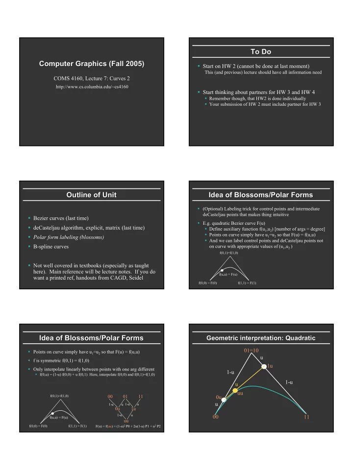
Idea of Blossoms/Polar Forms Idea of Blossoms/Polar Forms

Points on curve simply have u1=u2 so that F(u) = f(u,u) f is symmetric f(0,1) = f(1,0) Only interpolate linearly between points with one arg different

f(0,u) = (1-u) f(0,0) + u f(0,1) Here, interpolate f(0,0) and f(0,1)=f(1,0)

00 01 11

F(u) = f(uu) = (1-u)2 P0 + 2u(1-u) P1 + u2 P2 1-u 1-u u u 1-u u

0u 1u uu

f(0,0) = F(0) f(1,1) = F(1) f(0,1)=f(1,0) f(u,u) = F(u)

Geometric interpretation: Quadratic Geometric interpretation: Quadratic

u u u 1-u 1-u 00 01=10 11 0u 1u uu

SLIDE 2

Polar Forms: Cubic Bezier Curve Polar Forms: Cubic Bezier Curve

000 001 011 111 000 001 011 111

1-u u u u 1-u 1-u

00u 01u 11u

1-u u u 1-u

0uu 1uu

1-u u

uuu

Geometric Interpretation: Cubic

00u 0u1 u11 0uu uu1 uuu 000 111 001 011

Why Polar Forms? Why Polar Forms?

Simple mnemonic: which points to interpolate and how in deCasteljau algorithm Easy to see how to subdivide Bezier curve (next) which is useful for drawing recursively Generalizes to arbitrary spline curves (just label control points correctly instead of 00 01 11 for Bezier) Easy for many analyses (beyond scope of course)

Subdividing Bezier Curves Subdividing Bezier Curves

Drawing: Subdivide into halves (u = ½) Demo: hw2.exe

Recursively draw each piece At some tolerance, draw control polygon Trivial for Bezier curves (from deCasteljau algorithm): hence widely used for drawing

Why specific labels/ control points on left/right?

How do they follow from deCasteljau?

000 001 011 111 000 00u 0uu uuu uuu uu1 u11 111

Geometrically

00½ 0½1 ½11 0½½ ½½1 ½½½ 000 111 001 011

Geometrically

00½ 0½1 ½11 0½½ ½½1 ½½½ 000 111 001 011

SLIDE 3

Subdivision in Subdivision in deCasteljau deCasteljau diagram diagram

000 001 011 111 000 001 011 111

1-u u u u 1-u 1-u

00u 01u 11u

1-u u u 1-u

0uu 1uu

1-u u

uuu

Left part of Bezier curve (000, 00u, 0uu, uuu) Always left edge of deCasteljau pyramid Right part of Bezier curve (uuu, 1uu, 11u, 111) Always right edge of deCasteljau pyramid These (interior) points don’t appear in subdivided curves at all

Summary for HW 2 Summary for HW 2

Bezier2 (Bezier discussed last time) Given arbitrary degree Bezier curve, recursively subdivide for some levels, then draw control polygon hw2.exe Generate deCasteljau diagram; recursively call a routine with left edge and right edge of this diagram You are given some code structure; you essentially just need to compute appropriate control points for left, right

DeCasteljau DeCasteljau: Recursive Subdivision : Recursive Subdivision

DeCasteljau (from last lecture) for midpoint Followed by recursive calls using left, right parts

Outline of Unit Outline of Unit

Bezier curves (last time) deCasteljau algorithm, explicit, matrix (last time) Polar form labeling (blossoms) B-spline curves Not well covered in textbooks (especially as taught here). Main reference will be lecture notes. If you do want a printed ref, handouts from CAGD, Seidel

Bezier: Disadvantages Bezier: Disadvantages

Single piece, no local control (move a control point, whole curve changes) hw2.exe Complex shapes: can be very high degree, difficult In practice, combine many Bezier curve segments

But only position continuous at join since Bezier curves interpolate end-points (which match at segment boundaries) Unpleasant derivative (slope) discontinuities at end-points Can you see why this is an issue?

B B-

• Splines

Splines

Cubic B-splines have C2 continuity, local control 4 segments / control point, 4 control points/segment Knots where two segments join: Knotvector Knotvector uniform/non-uniform (we only consider uniform cubic B-splines, not general NURBS)

Knot: C2 continuity deBoor points

Demo: hw2.exe

SLIDE 4

Polar Forms: Cubic Polar Forms: Cubic Bspline Bspline Curve Curve

• 2 –1 0

–1 0 1 0 1 2 1 2 3

Labeling little different from in Bezier curve No interpolation of end-points like in Bezier Advantage of polar forms: easy to generalize

Uniform knot vector:

• 2, -1, 0, 1, 2 ,3

Labels correspond to this

deCasteljau deCasteljau: Cubic B : Cubic B-

• Splines

Splines

Easy to generalize using polar-form labels Impossible remember without

• 2 –1 0

–1 0 1 0 1 2 1 2 3

• 2 -1 0
• 1 0 1

0 1 2 1 2 3

• 1 0 u

0 1 u 1 2 u

? ? ? ? ? ?

deCasteljau deCasteljau: Cubic B : Cubic B-

• Splines

Splines

Easy to generalize using polar-form labels Impossible remember without

• 2 –1 0

–1 0 1 0 1 2 1 2 3

• 2 -1 0
• 1 0 1

0 1 2 1 2 3

• 1 0 u

0 1 u 1 2 u

1-u/3 (1-u)/3 (2+u)/3 (2-u)/3 (1+u)/3 u/3

0 u u 1 u u

? ? ? ?

deCasteljau deCasteljau: Cubic B : Cubic B-

• Splines

Splines

Easy to generalize using polar-form labels Impossible remember without

• 2 –1 0

–1 0 1 0 1 2 1 2 3

• 2 -1 0
• 1 0 1

0 1 2 1 2 3

• 1 0 u

0 1 u 1 2 u

1-u/3 (1-u)/3 (2+u)/3 (2-u)/3 (1+u)/3 u/3

0 u u 1 u u

(1-u)/2 (1+u)/2 1-u/2 u/2

u u u

1-u u

Explicit Formula (derive as exercise) Explicit Formula (derive as exercise)

• 2 -1 0
• 1 0 1

0 1 2 1 2 3

• 1 0 u

0 1 u 1 2 u

1-u/3 (1-u)/3 (2+u)/3 (2-u)/3 (1+u)/3 u/3

0 u u 1 u u

(1-u)/2 (1+u)/2 1-u/2 u/2

u u u

1-u u

3 2

1 ( ) [ 1] 2 3 P P F u u u u P P

M

      =      

1 3 3 1 3 6 3 3 3 1 4 1

1 6

M

− −     −     −    

=

P0 P1 P2 P3

Summary of HW 2 Summary of HW 2

BSpline Demo hw2.exe Arbitrary number of control points / segments

Do nothing till 4 control points (see demo) Number of segments = # cpts – 3

Segment A will have control pts A,A+1,A+2,A+3 Evaluate Bspline for each segment using 4 control points (at some number of locations, connect lines) Use either deCasteljau algorithm (like Bezier) or explicit form [matrix formula on previous slide] Questions?