This Lecture Physical Database Design RAID Arrays Efficiency and - - PDF document

SLIDE 1

1

Efficiency and Storage

Database Systems Michael Pound

This Lecture

• Physical Database Design
• RAID Arrays
• Parity
• Database File Structures
• Indexes
• Further reading
• The Manga Guide to Databases, Chapter 5
• Database Systems, Chapters 7, 18

Physical Design

• Design so far
• E/R modelling helps find

the requirements of a database

• Normalisation helps to

refine a design by removing data redundancy

• Next we need to think

about how the files will actually be arranged and stored

Project Description E/R Diagram Table Design Hardware Structure File Structure Physical Database Design

Physical Design

• Hardware
• Correct storage

hardware should be selected to avoid loss of data

• Speed can also be

affected by careful consideration of hardware

• RAID Arrays
• File Structure
• Often specifying the

structure of files on disks has a huge impact on performance

• Implementation of these

structures is also specific to a DBMS

• Indexes can be chosen to

further improve speed

RAID Arrays

• RAID - redundant array
• f independent

(inexpensive) disks

• Storing information

across more than one physical disk

• Speed - can access more

than one disk

• Robustness – disk failure

doesn’t always mean data is lost

• RAID Arrays are

controller by software

• r hardware
• At the OS level the RAID

array will appear to be a single storage device

• The array may actually

contain dozens of disks

• Different levels (RAID 0,

RAID 1,…)

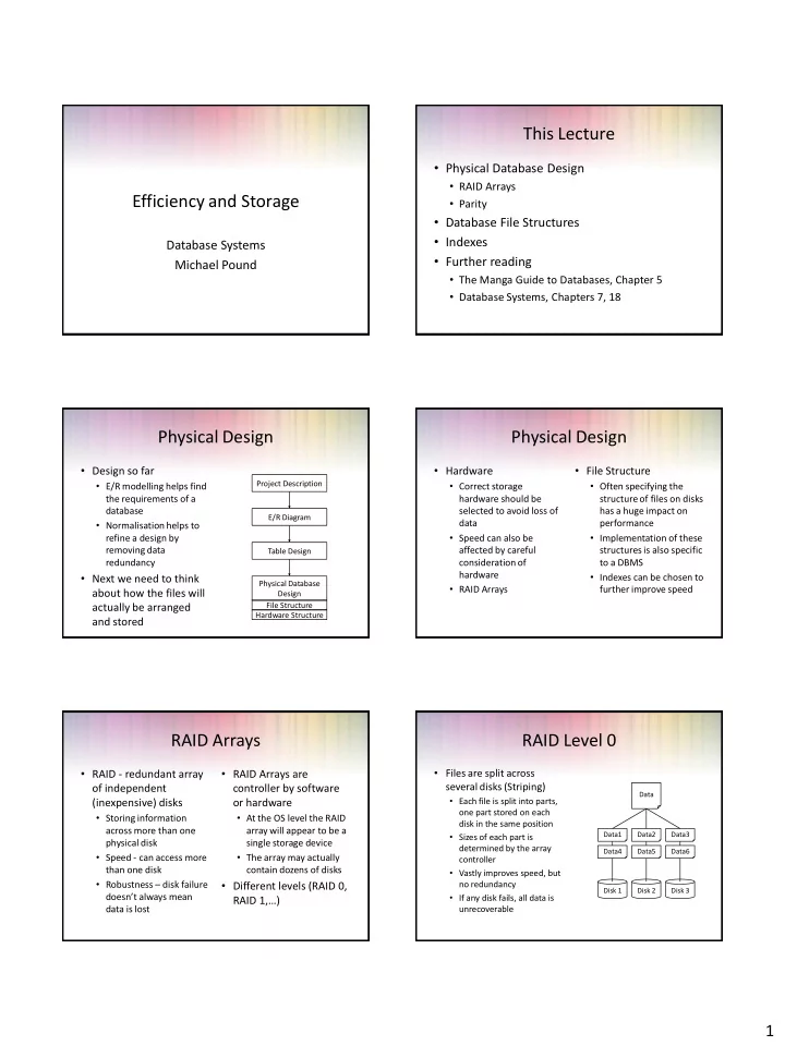
RAID Level 0

• Files are split across

several disks (Striping)

• Each file is split into parts,
• ne part stored on each

disk in the same position

• Sizes of each part is

determined by the array controller

• Vastly improves speed, but

no redundancy

• If any disk fails, all data is

unrecoverable

Disk 1 Data Data1 Data4 Disk 2 Data2 Data5 Disk 3 Data3 Data6

SLIDE 2

2

RAID Level 1

• Files are duplicated over

all disks (Mirroring)

• Each file is copied onto

every disk

• Provides improved read

performance but no write performance

• Large amounts of

redundancy, if all but a single disk fail the data can still be recovered

Disk 1 Data Data1 Data2 Disk 2 Data1 Data2 Disk 3 Data1 Data2

Parity Checking

• Above RAID 1 involves

calculating parity bits

• Parity reduces the

number of disks you need for redundancy

• Parity is often

calculated using XOR ⊕

• For two bits, A and B,

XOR is true if either A is true or B is true, but not both A B ⊕ 0 0 0 1 1 1 0 1 1 1

Parity Checking

• The parity of n blocks of data is calculated as

D1 ⊕ D2 ⊕ ... ⊕ Dn

• For example:

D1 0 0 1 1 0 1 1 0 D2 1 0 1 1 0 0 1 0 D3 1 1 0 0 0 0 0 0 DP 0 1 0 0 0 1 0 0

XOR is 0 if there is an even number of ‘1’ bits and 1 if there is an odd number

Recovery With Parity

• If any single disk breaks, including the parity

disk, XOR can be used to re-calculate that

• value. For example:

D1 0 0 1 1 0 1 1 0 D3 1 1 0 0 0 0 0 0 DP 0 1 0 0 0 1 0 0 D2 1 0 1 1 0 0 1 0

RAID Level 3

• Data is striped over

disks, and a parity disk for redundancy

• Data is split into bytes,

bytes are written to separate disks

• The final disk stores

parity information

• Extremely fast, and will

allow for 1 disk failure

Disk 1 Data Data1 Data4 Disk 2 Data 2 Data5 Disk 3 Data3 Data6 Disk 4 Parity(1-3) Parity(4-6)

RAID Level 5

• Data is striped over

disks with a distributed parity

• Data is split into blocks,

parity blocks are distributed throughout all disks

• Extended version of

RAID 3, and will even allow continued use after 1 disk failure

Disk 1 Data Disk 2 Disk 3 Data1 Data4 Data2 Data5 Data3 Data6 Data7 Data12 Data9 Data10 Data8 Data11 Disk 4 P(1-3) P(4-6) P(7-9) P(11-12)

SLIDE 3

3

Other RAID Issues

• Other RAID levels

consider

• Allowing more than a

single disk failure with the minimum of redundancy

• Nested RAID levels. For

example RAID 10 is a mirrored array of striped arrays

• Considerations with

RAID systems

• Cost of disks
• Do you need speed or

redundancy?

• How reliable are the

individual disks?

• ‘Hot swapping’

File Structure

• The structure of files on

a disk is separate to the RAID configuration

• File structure is

managed by the DBMS

• Often the designer of a

database can have control over aspects of this structure

• In general file structure

is concerned with:

• How files are stored on a

disk

• In what order files are

stored

• The speed at which a file

can be retrieved

• The speed at which files

can be inserted or deleted

Pages and Rows

• Row data is generally

not written to disk

• individually. Instead,

rows are grouped into pages

• Pages are often used as

the atomic unit of I/O, any read or write to the disks will be a page, even if only a single row is affected

• A page will include a

header and the row data:

• There are usually many

rows in a page, but not always

Page Header Row 1 Row 2 Row 3 Row 4 Row 5

Pages and Rows

• A table will often span

multiple pages

• INSERTs will be added at

the last position in the newest page

• Additional pages can be

added if the previous

• ne is full
• For a student table:

Page 1 11011465 Jack ... 1 11011658 Robert ... 2 11044348 Sarah ... 3 11051499 Max ... 1 Page 2 11012234 James ... 2 11034868 Mike ... 2 11048345 Anne ... 1

Unordered Files

• Unordered files are often

called Heaps

• New records are inserted

into the last page of the file

• If the page is full, a new

page is added at the end

• f the file
• This structure makes

insertion very efficient

• There is no ordering on

values however, so searching must be conducted linearly

• To delete a record, the

page is retrieved, a row is marked as deleted, and the page is written back

• This space is difficult to

reclaim, so performance will deteriorate over time

Ordered Files

• Data sorted by one or

more fields is called a sequential file

• Inserting and deleting

from an ordered file is difficult

• If there is sufficient

space on the correct page, a record can be inserted and that page re-written

• Full pages can

propagate along and require many rewrites

• One solution is to

temporarily add records to an overflow file, these are merged at a later time

• Overflows improve

inserts, but make searches more difficult

SLIDE 4

4

Binary Search

• A huge benefit of an
• rdered data structure

is the concept of the binary search

• A binary search is only

possible when searching for specific values in a field, where the data is also ordered by that field

• Consider the Student

table, ordered by sID:

SELECT * FROM Student WHERE sID = 11062365;

• A linear search through

the database could involve thousands of reads

Binary Search

Searching for: 11062365

• We begin the search by

retrieving the page half way through the file

• The ID values in the

page are smaller than the one we're looking for so we next look further down the file

Data Rows Page 11010001 ... 1 11011123 ... 2 11023134 ... 3 11025421 ... 4 11031341 ... 5 11034342 ... 6 11045332 ... 7 11058543 ... 8 11062365 ... 9 11072234 ... 10 11074122 ... 11 11077898 ... 12 11082232 ... 13 11083239 ... 14

Binary Search

Searching for: 11062365

• We next retrieve the

page half way through the remaining half that contains our value

• The values are larger

than the ID we are looking for, so we must travel backwards in the file

Data Rows Page 11010001 ... 1 11011123 ... 2 11023134 ... 3 11025421 ... 4 11031341 ... 5 11034342 ... 6 11045332 ... 7 11058543 ... 8 11062365 ... 9 11072234 ... 10 11074122 ... 11 11077898 ... 12 11082232 ... 13 11083239 ... 14

Binary Search

Searching for: 11062365

• We retrieve the page

half way between the two previous pages

• The value we are

looking for is on this

• page. We read the

remaining row data

• Binary searches

complete in Log2n time, which is often better than a linear search

Data Rows Page 11010001 ... 1 11011123 ... 2 11023134 ... 3 11025421 ... 4 11031341 ... 5 11034342 ... 6 11045332 ... 7 11058543 ... 8 11062365 ... 9 11072234 ... 10 11074122 ... 11 11077898 ... 12 11082232 ... 13 11083239 ... 14

Indexes

• Strictly speaking, the

relational model states that the ordering of tuples does not matter

• In reality this is

inefficient, searching and ordering are much easier using sequential files

• We can obtain further

improvements with indexes

• An Index is a data

structure that resides alongside a table, providing faster access to the rows

• An Index is associated

with one of more fields, improving searches involving those fields

• The underlying data

may or may not be

• rdered

Indexes

• Indexes are not unlike

those you find in books

• The aim is to simplify the

search for key words or values

• Often much faster than

looking through the book linearly

• The index will be
• rdered to improve

search efficiency

• There are a number of

types indexes

• Primary indexes refer to

a sequential file ordered by a key (unique)

• Clustered indexes refer

to a sequential file

• rdered by some fields

that may not be unique

• Secondary indexes exists

separately to the data

• rdering

SLIDE 5

5

Spares and Dense Indexes

• Indexes can be broadly split into two categories, sparse and

dense indexes

• Dense indexes contain a value matching every row
• Take up more memory but don’t require the data to be sorted

Data Rows Page 11010001 Jack … 1 11011123 Sarah … 11023134 Robert … 2 11025421 James … 11031341 Mike … 3 11034342 Anne … 11045526 Tony … 4 11046245 Nick … Index Anne 3 Jack 1 James 2 Mike 3 Nick 4 Robert 2 Sarah 1 Tony 4

Spares and Dense Indexes

• Indexes can be broadly split into two categories, sparse and

dense indexes

• Sparse indexes only match a subset of the rows
• Efficient searches using a spare index need to be on a sequential file

Data Rows Page 11010001 Jack … 1 11011123 Sarah … 11023134 Robert … 2 11025421 James … 11031341 Mike … 3 11034342 Anne … 11045526 Tony … 4 11046245 Nick … Index 11011123 1 11025421 2 11034342 3 11046245 4

Benefits of Indexing

• Sparse indexes significantly reduce the

number of page reads required to retrieve the specific page a search requires

• Indexes are often stored in memory to further

improve search speed

• However, every index must be maintained,

and this adds complexity to INSERT, UPDATE and DELETE queries

Multi-level Indexes

• It’s possible, and often beneficial, to add higher levels of

sparse index above existing ones

• Higher levels contain fewer index rows, and point you towards

less sparse indexes lower down

• The final level points you towards the table data

Data Rows Page 11010001 Jack … 1 11011123 Sarah … 11023134 Robert … 2 11025421 James … 11031341 Mike … 3 11034342 Anne … 11045526 Tony … 4 11046245 Nick … Index Level 2 11011123 1 11025421 2 11034342 3 11046245 4 Index Level 1 11025421 1 11046245 2

ISAM

• ISAM stands for Indexed Sequential Access Method
• Essentially a static, sparse, often multi level primary index
• The lowest level index points to anchor rows that

represent each page. The index always references pages, rather than specific rows

• Pages are linked together either by being consecutively

stored on disk, or each page holds a pointer to the next

• ne. This means values can be read sequentially extremely

fast

• Because the index is static, it must be reorganised
• ccasionally to prevent a deterioration in speed
• ISAM is less suitable for databases with very frequent

inserts or deletes. Overflow areas are used if necessary

ISAM

• A 2-level ISAM Index for the Student table

11010001 Jack … 11011123 Sarah … 11023134 Robert … 11025421 James … 11045526 Tony … 11046245 Nick … 11010001

• ⁞

11023134

• ⁞

11031341

• 11045526
• ⁞

⁞ 11010001

• ⁞

11030001

• 11031341

Mike … 11034342 Anne … ⁞

SLIDE 6

6

B+-Trees

• B-Trees are balanced tree structures, and are now the most

common method for indexing in databases. They are used as a dense index

• A balanced tree is a hierarchy of nodes each of which links to child

nodes below it, much like ISAM

• The top of the tree is the root, nodes with no children are called

leaf nodes. Leaf nodes are interconnected for sequential access

• An example node would look like this:
• Key Value 1

Key Value 2 Child Node Child Node Child Node or Next Leaf

Example B+-Tree

• An example B+-Tree Index for the Student table
• 11010001

11011123

• 11023134
• 11031341

11034342

• 11045526
• 11011123
• 11034342
• 11023134
• Benefits of B+-Trees
• B-Trees vastly reduce the number of reads

necessary to access a specific database row

• For example, if the order (the number of allowed

children) is 256, then a single row in a database of 16million rows could be accessed with 4 disc reads

• Inserts and Deletes usually require the tree nodes

to be slightly rearranged to balance the tree. This is an efficient procedure, but we will not cover it in this module

Clustered Indexes

• In many modern DBMSs, rather than the leaf

nodes of a B+-tree pointing to the locations of the data rows, the leaf nodes themselves are adapted to hold the row data

• This reduces a read operation where the row has to

be looked up

• This adapted B+-tree is often called a clustered index

and is the default storage structure in InnoDB and

• ther DBMSs
• By default, a table in InnoDB will be a clustered index
• n the primary key

Choosing Indexes

• You can only have one

primary or clustered index

• The most frequently

looked-up value is often the best choice

• Some DBMSs assume

the primary key is the primary index, as it is usually used to refer to rowss

• Don’t create too many

indexes

• They can speed up queries,

but they slow down inserts, updates and deletes

• Whenever the data is

changed, the index may need to change

• Create secondary indexes

if another field might

• ften be used for
• rdering or searching

Creating Indexes

• In SQL we use CREATE

INDEX:

CREATE INDEX <index name> ON <table> (<columns>)

• Example:

CREATE INDEX sIndex ON Student(sName); CREATE INDEX smIndex ON Student (sName, sMark);

SLIDE 7

7

Next Lecture

• Database Security
• Privileges
• GRANT and REVOKE
• SQL Injection Attacks
• How to write an injection attack
• How to secure your system against them
• For more information
• The Manga Guide to Databases, Chapter 5
• Database Systems, Chapter 7