
SLIDE 1
The Physical Pendulum and the Onset of Chaos
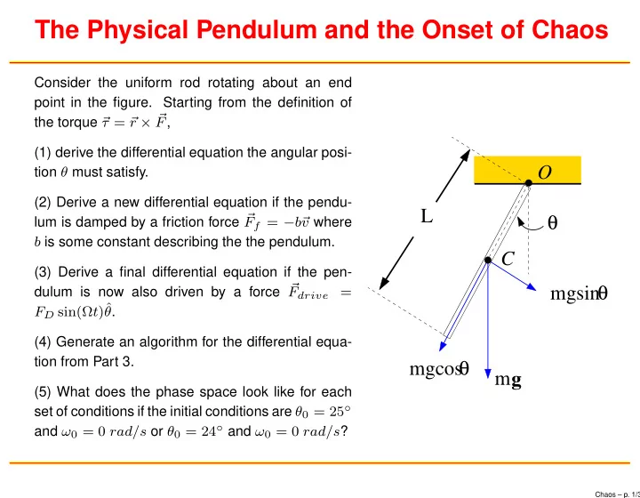
Consider the uniform rod rotating about an end point in the figure. Starting from the definition of the torque τ = r × F, (1) derive the differential equation the angular posi- tion θ must satisfy. (2) Derive a new differential equation if the pendu- lum is damped by a friction force Ff = −b v where b is some constant describing the the pendulum. (3) Derive a final differential equation if the pen- dulum is now also driven by a force Fdrive = FD sin(Ωt)ˆ θ. (4) Generate an algorithm for the differential equa- tion from Part 3. (5) What does the phase space look like for each set of conditions if the initial conditions are θ0 = 25◦ and ω0 = 0 rad/s or θ0 = 24◦ and ω0 = 0 rad/s?
m mgsin θ g θ O C mgcos θ L
Chaos – p. 1/3