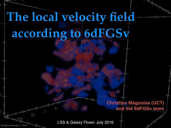
The local velocity field according to 6dFGSv Christina Magoulas - PowerPoint PPT Presentation

The local velocity field according to 6dFGSv Christina Magoulas (UCT) ! and the 6dFGSv team LSS & Galaxy Flows: July 2016 Background Image: C. Fluke

6dFGSv: outline 6dFGSv: distances and peculiar velocities • defining the 6dFGSv sample and the individual peculiar velocity distributions. 6dFGSv: the most recent results • cosmological constraints from the velocity power spectrum (Johnson et al. 2014) and MV bulk flow (Scrimgeour et al. 2016). 6dFGSv: cosmographic results • 3D map of the velocity field out to 160 Mpc/h, as traced by 6dFGSv Maximum Likelihood forward fitting of the bulk flow and β • Bayesian analysis of the 6dFGSv dataset as a whole

The 6dF peculiar velocity survey (6dFGSv) • 6dFGS: combined redshift (z-) and peculiar velocity (v-) survey of the entire Southern Sky on the UK Schmidt Telescope; large uniformly sampled volume -1 • 6dFGSv: 9000 peculiar velocities using FP distances out to cz<16000 km s • Largest homogeneous velocity survey to date

Peculiar Velocity Distributions • For each galaxy we determine individual probability distributions in log (distance ratio) units where errors are Gaussian , taking advantage of (forward) fitting in “data” space Gaussian distribution in log(distance) space where x = log 10 (D z /D H ) skewed in velocity, v p , distribution (errors are close to log-normal ) Johnson et al. MNRAS (2014)

6dFGSv distance and velocity data From Springob et al. MNRAS (2014) • redshifts (cz), log distance ratios ( Δ d), and probability distribution variables ( ϵ d , ⍺ ) available online: http://vizier.cfa.harvard.edu/viz-bin/ VizieR?-source=J/MNRAS/445/2677 Springob et al. MNRAS (2014)

6dFGSv: survey papers • Springob et al. 2014: The 6dF Galaxy Survey: peculiar velocity field and cosmography. • Johnson et al. 2014: The 6dF Galaxy Survey: cosmological constraints from the velocity power spectrum. • Scrimgeour et al. 2016: The 6dF Galaxy Survey: bulk flows on 50-70 h -1 Mpc scales. • Magoulas et al. (THIS TALK): The 6dF Galaxy Survey: bulk flows and β from fitting the peculiar velocity field

• Johnson et al. 2014: Constraining the growth rate of structure using a velocity power spectrum analysis of 6dFGSv and SNe data Λ CDM prediction Johnson et al. MNRAS (2014)

f σ 8 (z = 0) = 0.418±0.065 Λ CDM prediction (Planck) 300 Mpc/h 100 Mpc/h 50 Mpc/h Johnson et al. MNRAS (2014) • Redshift zero measurement of the growth rate that is independent of galaxy bias and accurate to ~15% • sensitive to largest scales; consistent with fiducial Planck cosmology See also Howlett talk tomorrow

• Scrimgeour et al. 2016: using a minimum variance method to measure the 6dFGSv bulk flow in Gaussian spheres of R I =50 and 70 h -1 Mpc • At R I =50 h -1 Mpc: |U| = 248±58 km s -1 (l,b) = (318°±20°, 40°±13°) • At R I =70 h -1 Mpc: |U| = 243±58 km s -1 (l,b) = (318°±30°, 39°±13°) • Largest discrepancy in z-direction when compared to MLE method (reflects difference in weighting schemes)

Λ CDM prediction (all-sky Gaussian window) Scrimgeour et al. MNRAS (2016) • Scrimgeour (2016) bulk flow in agreement with recent measurements: Turnbull et al. (2012), Feindt et al. (2013), Hong et al. (2014) • Somewhat higher bulk flow than Λ CDM prediction on these scales, implying a high value of σ 8 , but consistent with Planck results within 2 σ

Peculiar Velocity Fitting Method • We have two choices: [1] Forward-fitting (Magoulas et al. in prep.) Fitting model to the data and compare in “data space”. Do a Bayesian analysis of the observational data set as a whole (in r-s-i space), without computing individual peculiar velocities. ! [2] Reverse-fitting (Springob et al. 2014) Fitting data to the model and compare in “model space”. Compute a Bayesian posterior probability distribution for the distance/ peculiar velocity of each galaxy, rather than a single velocity.

Smoothed 3D 6dFGSv velocity field 3D Visualisation by S2PLOT Springob et al. (2014)

3D map of 6dFGSv velocity field (smoothed) showing only those regions with largest positive/negative velocities 3D Visualisation by S2PLOT Springob et al. (2014)

Cosmicflows-2 > 3: slice in the Supergalactic equatorial plane CF-2: Tully et al. (2014) Addition of 6dFGSv (orange) is significant fraction of the South CF-3: Tully et al. (submitted)

• Distance ratio along LOS within 30° of local structure compared with models of 2MRS and PSCz • Systematically 2MRS positive peculiar velocities in vicinity of Shapley (as well as Norma and Vela Supercluster) • Offset by more negative than expected peculiar velocities in the direction of Pisces- PSCz Cetus Supercluster, ( ∼ 130° away) Springob et al. (2014)

• The 6dFGSv bulk flow is 395±64 km s -1 in the direction (l,b) = (318°±20°, 40°±13°) using ML forward modeling approach 16000 75 � 60 � 14000 45 � 6dFGSv 30 � 12000 CMB 15 � cz [km s − 1 ] 10000 90 � 60 � 30 � 0 � 330 � 300 � 270 � 240 � 210 � 180 � 150 � 0 � 8000 -15 � 6000 -30 � 4000 -45 � -60 � 2000 -75 � 6dFGSv (total) Turnbull et al. 2012 (total - ML) Colin et al. 2011 6dFGSv (residual) Turnbull et al. 2012 (residual) Dai et al. 2011 Watkins et al. 2009 Turnbull et al. 2012 (total - MV) Nusser & Davis 2011

6dFGSv flow as a function of scale Magoulas et al. (in prep) • Different surveys have 800 different window functions; hard to compare with each CMB 600 other or predictions. | v tot | [km s − 1 ] COMPOSITE 6dFGSv • Selection function reduces the 400 6dFGSv effective volume of the survey ND11 CMSS11 A1 DKS11 200 0 0 50 100 150 R [ h − 1 Mpc] Scrimgeour et al. MNRAS (2016)

Velocity model reconstruction • Reconstruction of the density and velocity field (following the linear theory -1 Mpc; based on the all-sky method of Carrick et al. 2015) within 200 h 2M++ redshift catalogue (mostly 6dF in the South) 2M++ density field 2M++ velocity field Carrick et al. 2015 Carrick et al. 2015, Magoulas et al. in prep. 0.55 /b). • Velocity field determined by the linear redshift-space distortion parameter, β (= Ω m

Beta and external dipole results • The beta parameter is consistent with recent results when 6dFGSv is compared to 2MRS ( β fid =0.4) and PSCz ( β fid =0.5), but low when compared to 2M++ ( β fid =0.43) • We measure large external bulk flows (assuming matter follows the galaxy distribution of the model reconstruction) but largest with comparison to 2M++ 420±65 km/s with a very low β =0.18±0.05; • amplitude is not too much smaller than total flow! (u tot =395±64).

v-v chi-squared fitting • Simple linear regression ( χ 2 ) to individual log 10 (D z /D H ) ratios as an independent check to 2M++ (doesn’t account for sample selection, distance weighting, zero-point calibration) • From this method, best-fit of β = 0.13 is consistently close to the value fitted by the full ML forward modeling (cf. β = 0.14±0.06) and suggests usual fitting method is robust. • Hence there still exists a large discrepancy between the observed 6dFGSv and predicted 2M++ velocities.

Summary • 6dFGSv provides the largest homogenous sample of galaxy peculiar velocities to date. • We model the velocity field and 3D FP Gaussian simultaneously using a Bayesian analysis of the dataset as whole. Using 6dFGSv, we map the velocity field in the nearby universe and compare to the density field derived from redshift surveys. • This leads to new measurements on the redshift distortion parameter with some discrepancies: β =0.32±0.08 (2MRS), β =0.58±0.12 (PSCz) and β =0.13±0.06 (2M++) • We recover a total bulk flow for 6dFGSv within ~160 Mpc/h of 395±64 km/s towards (l,b) = (318˚±20˚, 40˚±13˚) meaning the 6dFGSv volume has a substantial coherent motion towards Shapley .

Thank You

6dFGSv velocity field in 30 Mpc/h spheres around local overdensities 3D Visualisation by S2PLOT Springob et al. (2014)

morphology outliers • Log distance ratio versus morphological type separated by morphological subsamples (top; early types in red, intermediate types in green, late types in blue) and full sample (bottom). • The median bins (with rms error bars) indicate that a cut of T > 3 removes the most discrepant outliers,

6dFGSv flow as a function of scale T O P H AT F I LT E R ( 9 0 % P R O B A B I L I T Y ) ! 800 G A U S S I A N F I LT E R ( 9 0 % P R O B A B I L I T Y ) CMB radius of sphere with 600 same volume as | v tot | [km s − 1 ] 6dFGSv 6dFGSv “hemisphere” survey limit COMPOSITE 6dFGSv 400 6dFGSv ND11 CMSS11 A1 DKS11 200 0 0 50 100 150 R [ h − 1 Mpc] • There is still disagreement between surveys at similar scales (Watkins 2009; Nusser & Davis 2011) and with standard model predictions (Colin 2011, Watkins 2009)