v v cr = E B to pass through. F E v < v cr Lec27-2 Velocity - PowerPoint PPT Presentation

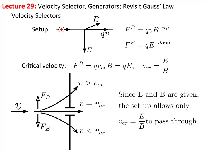
Lecture ¡29: ¡ Velocity ¡Selector, ¡Generators; ¡Revisit ¡Gauss’ ¡Law ¡ Velocity ¡Selectors ¡ B Setup: ¡ F B = qvB up qv F E = qE down E v cr = E Cri;cal ¡velocity: ¡ F B = qv cr B = qE, B v > v cr Since E and B are given, F B v = v cr the set up allows only v v cr = E B to pass through. F E v < v cr

Lec27-2 Velocity selector-2 fig 27 . 1 y v x q E z If the sign of the charge q is negative , what is the direction of B in order to reproduce the non-deflection condition? Choice Direction of B 1 Into 2 Out

Sliding ¡bar ¡along ¡2 ¡|| ¡conduc;ng ¡rails. ¡ F N A qv qv Polarized Charges E pol B B Magne;c ¡Force ¡is ¡pushing ¡posi;ve ¡test ¡charge ¡uphill ¡ ∴ emf = W A → B = qvBh = vBh q q ? Mechanical Power = Fv = Power of dissipation = E I ( IhB ) v = ( vBh ) I E R Conservation of Energy

Rota;ng ¡Disk ¡ A B qv F M E pol B ~ E pol : Define the direction of down hill to be from B to A. Magnetic Force F M pushes positive charge from A to B. Compare ¡the ¡poten;als: ¡ V A vs. V B 1. ¡ 2. ¡ V A < V B V A > V B

Rota;ng ¡Loop ¡induces ¡emf ¡in ¡the ¡loop ¡ Top View: ω v = ω r v ⊥ v B h P v k ~ v × ~ F = q ~ B | F | = qv ⊥ B Max occurs at P: F max = qvB emf max = F max h = vBh = ω RBh. q ω is in units of rev min = rev min · 2 π rev

Current ¡loop ¡in ¡motors ¡and ¡generators ¡ We ¡recall ¡that ¡a ¡current ¡loop ¡generates ¡a ¡magne;c ¡field. ¡ B z ∝ 1 RHR-­‑5 ¡ z 3 ⌘ 2 I π 2 R ⇣ µ 0 n µ loop = IA ˆ B z = loop z 3 4 π A ¡current ¡loop ¡is ¡equivalent ¡to ¡a ¡magnet. ¡ I Loop-­‑magnet, ¡density ¡ B ¡exerts ¡a ¡torque ¡on ¡the ¡emf ¡loop ¡ F µ × ~ ~ ⌧ = ~ B With ¡a ¡split ¡ring ¡arrangement, ¡the ¡loop ¡ B can ¡rotate ¡endlessly ¡– ¡this ¡is ¡the ¡principle ¡ F behind ¡a ¡motor. ¡

Rota;ng ¡loop ¡generates ¡emf ¡in ¡a ¡loop ¡ Max ¡emf ¡is ¡when ¡B ¡aligns ¡with ¡the ¡ v b plane ¡of ¡the ¡loop ¡(rectangle ¡a ¡x ¡b) ¡ B E max = 2 qvBb F = qvB q a = 2 vBb = 2 a 2 Bb = ω abB E loop E = ( ω abB ) sin ω t

Beyond ¡symmetric ¡applica;on ¡of ¡Gauss ¡Law ¡and ¡Ampere’s ¡Law ¡ Q 4 ⇡ r 2 E = Q 1 Gauss ¡Law: ¡Point ¡charge ¡ E = r 2 , 4 ⇡✏ 0 ✏ 0 A = Q S I E · d ~ ~ General ¡Form: ¡ ✏ 0 S S ¡can ¡be ¡arbitrary, ¡Q S ¡any ¡charge ¡distribu;on ¡enclosed ¡by ¡S ¡ 4 ⇡ r 2 E = Q ✏ 0 2 AE = Q ✏ 0 2 ⇡ rhE = Q ✏ 0

Begin ¡with ¡1 ¡point ¡charge ¡q ¡with ¡arbitrary ¡surface ¡S ¡which ¡encloses ¡q ¡ · q 1 E 1 A 1 = r · A 1 ˆ r 2 4 ⇡✏ 0 1 A 1 A 2 r 1 r ∆Ω = ˆ r 2 · A r 2 1 E 2 A 2 = q ∆Ω 4 ⇡✏ 0 ∆Ω = q 1 I I Over ¡enclosing ¡surface: ¡ LHS = q ∆Ω = 4 π 4 ⇡✏ 0 ✏ 0 X q ( k ) Let: Q s = k P k q k I Super ¡posi;on: ¡ E ( k ) · dA = ✏ 0

q fig. 29-1 A charge q is placed at the corner of the cube shown in fig29.1. Find the electric flux through the shaded area. Choice � shaded 1 q / (6 / ✏ 0 ) 2 q / (12 / ✏ 0 ) 3 q / (24 / ✏ 0 ) 4 q / (36 / ✏ 0 )

Total ¡flux: ¡ q ✏ 0 Through ¡1 ¡cube: ¡ × 1 8 Through ¡1 ¡face: ¡ × 1 3 × 1 ∴ Flux through shaded square face: q 24 ✏ 0

Lec29-3 Beyond symmetric charged distributions-III q − Q C fig29.3a A metal block containing a cavity and carrying a net charge − Q is located near a positive charge q as shown in fig. 29.3a. For a static situation, can there be charges on the surface C of the cavity? Choice Charges on the surface C ? 1 Yes 2 No

Lec29-4 Beyond symmetric charged distributions-IV Fig. 29.4 shows an empty metal box located near a positive charge q . q causes the metal box to polarize, producing the surface charge distribution shown. Determine the electric field at a point inside of the metal box near the upper right hand corner. Choice E-field near the right-upper corner of the block 1 E is pointing towards from + q 2 E is pointing away from + q 3 E = 0

Field ¡near ¡the ¡surface ¡of ¡a ¡conductor ¡ Gauss ¡Law: ¡ E ⊥ E ⊥ ∆ A = ∆ Q surface ✏ 0 E ⊥ = � surface ✏ 0 Theorem: E ⊥ ⇔ ∆ Q surface / ∆ A ✏ 0 So ¡once ¡E-­‑perpendicular ¡is ¡given, ¡the ¡corresponding ¡surface ¡charge ¡density ¡ is ¡determined. ¡ ¡ Conversely, ¡once ¡the ¡surface ¡charge ¡density ¡is ¡given ¡E-­‑perpendicular ¡can ¡be ¡ determined. ¡

Applica;on: ¡Determine ¡surface ¡charge ¡by ¡reflec;on ¡ +Q -Q Inner ¡Charges: ¡ Outer ¡Charges: ¡ +Q -Q 0 E = 0 E = 0 +Q -Q ∴ E gap = Q/A ✏ 0

+5Q -3Q +2Q +5Q -3Q +Q +Q +Q +4Q -4Q +Q ∴ E gap = 4 Q/A ✏ 0