
SLIDE 1
The Initial Core Mass Function Near and Far
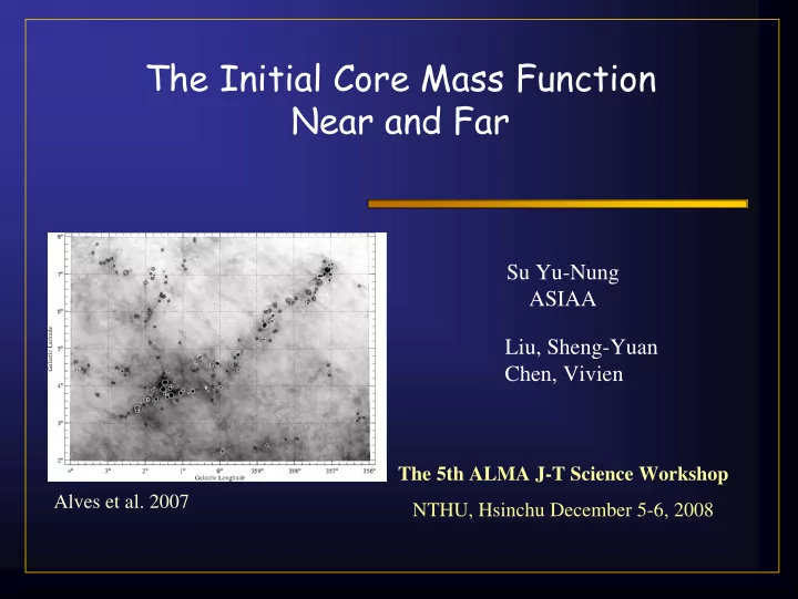
Su Yu-Nung ASIAA
The 5th ALMA J-T Science Workshop NTHU, Hsinchu December 5-6, 2008
Liu, Sheng-Yuan Chen, Vivien
Alves et al. 2007
The Initial Core Mass Function Near and Far Su Yu-Nung ASIAA Liu, - - PowerPoint PPT Presentation
The Initial Core Mass Function Near and Far Su Yu-Nung ASIAA Liu, Sheng-Yuan Chen, Vivien The 5th ALMA J-T Science Workshop Alves et al. 2007 NTHU, Hsinchu December 5-6, 2008 Outline Background & Motivation Initial mass
Su Yu-Nung ASIAA
The 5th ALMA J-T Science Workshop NTHU, Hsinchu December 5-6, 2008
Liu, Sheng-Yuan Chen, Vivien
Alves et al. 2007
dN/dM ~ M-α α = 2.35 – 2.7 for star mass > 0.6-1 M⊙
(Salpeter 1955, Miller & Scalo 1979, Kroupa 2002, Muench et al. 2002)
– Nevertheless, the origin the stellar IMF remains one of the major unsolved problems in modern astrophysics. – Since stars form in molecular clouds, the knowledge of mass spectrum of molecular cloud cores is likely a key for understanding the origin of the IMF
– Observations of nearby star forming regions
– Serpens, Testi & Sargent 1998 – Orion A, Johnstone & Bally 1999, 2006 – Orion B, Johnstone et al. 2001, 2006 – ρ Ophiuchus, Motte et al. 1998, Johnstone et al. 2000 – NGC 2068/2071, Motte et al. 2001
– nearby clouds, C18O, Tachihara et al. 2002 – Taurus, H13CO+, Onishi et al. 2002 – Orion A, H13CO+, Ikeda et al. 2007
– Pipe dark cloud, Alves et al. 2007
The dense core mass function derived from near-IR extinction map in the Pipe dark cloud (Alves et al. 2007)
the IMF
higher masses
the dense core mass function
efficiency of ~ 30%
Similar power indices have been identified by mm/sub-mm continuum as well as molecular line surveys
The location of the break is similar to that of IMF (Motte et al. 1998; 2001) Incompleteness sample at low-mass end (Testi et al. 1998, Johnstone et al. 2001) Lack of identification of “massive cores” (Motte et al. 2001)
Testi & Sargent 1998
Serpen
Pipe dark cloud
(Alves et al. 2007) Motte et al. 2001
NGC 2068/2071
The Connection Between Cloud Structure and the IMF
Science goal: The origin of the IMF and its relationship to the initial conditions within star forming molecular clouds is one of the major unsolved problems in star formation, and one which has implications for almost every scientific field in which ALMA will be important. We propose to conduct a large-scale survey of the Ophiuchus, Lupus, Perseus, and Orion molecular cloud complexes in order to determine this relationship. The main survey will be carried out at 1 mm, and companion survey at 3 mm is needed to enable us to distinguish unambiguously between dust and free-free emission. Number of sources: 4 (Ophiuchus, Perseus, Lupus, and Orion) Total integration time: 400 hrs
5.1. Angular resolution: 1" 5.2. Range of spatial scales/FOV: 1 degree 5.3. Single dish: yes 5.4. ACA: yes 5.5. Subarrays: no
6.1. Receiver band: Band 6 230 GHz and Band 3 100 GHz
7.1. Typical value: 1 mJy 7.2. Continuum peak value: 1 Jy 7.3. Required continuum rms: 0.3 mJy 7.4. Dynamic range in image: 1000
4 x 6 s x 57600 fields at 230 GHz 4 x 1 s x 14400 fields at 100 GHz (NOTE: use OTF mosaicing)
– Cloud @ 2kpc – 6 pc x 3 pc (comparable to OMC 1,2,3, and 4) – 600’’ x 300’’ – Observations 230 GHz – Rms 0.54 mJy (= 5 sigma mass detection for 0.3 M☉ sources) – Total integration time : 38 mins (2.15 s x 1050 field)
(http://www.eso.org/sci/facilities/alma/observing/tools/etc/index.html)
For the same rms (in terms
Jy), the integration time ratio ~ 1 : 5 : 20 : 170 for observations at 100, 230, 345, and 690 GHz) high-freq. is slow Field number ∝ ν2 high freq. will be even slow Observations at 650 GHz band are much slower than that at 100 GHz band!! Observations at 3-mm are fastest III IV V VI VII VIII IX
But for obs. at different frequency, the required rms noise levels are not same. What we need is the same mass detection limit. for β=0, flux ~ ν2 rms ~ ν2 integration time ~ ν-4 Obs @ 230 GHz is the most efficient, but only a factor of 5 faster than
for β=0.5, rms ~ ν2.5 integration time ~ ν-5 for β=1.0, rms ~ ν3 integration time ~ ν-6 High-freq is better !! For β=1.0, obs @ 650 band is the fastest
for β=1.5, rms ~ ν3.5 integration time ~ ν-7 for β=2.0, rms ~ ν4 integration time ~ ν-8 for β=2, observations @ 680 GHz, the required total integration time is
(2kpc, 6 pc x 3 pc, 5 sigma detection limit of 0.3 M⊙ sources)
single field: for the same mass detection limit (F ~ M/d2) rms noise level ~ 1/d2 integration time ~ d4 Field Number for the same physical area filed number ~ d-2 Nearer is faster Total integration time ~ d2 2 kpc : 2 mins (0.014 s / field) 20 kpc : 200 mins (137 s / field) 50 kpc : 1250 mins = 21 hrs (90 m / field)
– Resolution, largest and smallest scales ?? – Can we have such a “short” integration time ??
– Dynamical Range ??
– Given large mosaic fields, can we obtain “uniform” map ??
Aboved-mention conclusions (i.e., 680 GHz is the fastest, and nearer is faster) are based on the assumption of point-like structure. Such assumption, however, may not be valid Dense core size : 2,000 – 10,000 AU 1”-5” @ 2kpc
(Motte et al. 1998, 2001)
Band frequency range (GHz) angular resolution bmax=200m ... 18km (arcsec) line sensitivity (mJy) continuum sensitivity (mJy) primary beam (arcsec) largest scale (arcsec) 3 84-116 3.0 ... 0.034 8.9 0.060 56 37 4 125-169 2.1 ... 0.023 9.1 0.070 48 32 5 163-211 1.6 ... 0.018 150 1.3 35 23 6 211-275 1.3 ... 0.014 13 0.14 27 18 7 275-373 1.0 ... 0.011 21 0.25 18 12 8 385-500 0.7 ... 0.008 63 0.86 12 9 9 602-720 0.5 ... 0.005 80 1.3 9 6
http://www.eso.org/sci/facilities/alma/observing/specifications/
For sources at 2 kpc, even the most compact one will be resolved with ALMA observations at high-freq. (>400 GHz) bands
For sources at distance > 4kpc, the two conclusions are likely valid if the less massive sources have smaller sizes Although the brighter sources can be well resolved, sensitivity is unlikely an issue if applying taper weighting Assuming uniform uv coverage (visibility number / uv area ~ const) Rms ~ beam size using uv < 0.1 x bmax beam size x 10 rms x 10 mass limit x 10
10000 AU 2000 AU
For sources at distance > 4 kpc, observations @ 680 GHz are the most efficient.
The required integration time for a single field : β=1 1.92 x (d/4kpc)4 sec β=2 0.22 x (d/4kpc)4 sec Total integration time: (6 pc x 3 pc, field number~ 2200 (d/4kpc)-2) β=1 70 x (d/4kpc)2 min β=2 8 x (d/4kpc)2 min
For sources located within 4 kpc, we have to reexamine the two
integration time and source distance ? for sources with the same mass total flux ~ d-2 + source angular size ~ d-1 constant brightness required rms level not related to distance but for mapping the same physical scale, mosaic field number ~ d-2 farther is faster !!
For sources with d < 4 kpc, we have to reexamine the two conclusions.
(i.e., 680 GHz is the fastest, and nearer is faster)
integration time and source distance ? for sources with the same mass total flux ~ d-2 source angular size ~ d-1 if applying taper weighting rms ~ d-1 integration time ~ d2 but field number ~ d-2
total integration time cont. over source distance 4 kpc, 0.5”, 5 mJy, rms 1mJy 5 simga 2 kpc, 1’’, 20 mJy resolution 0.5”, rms 2mJy taper 1.0”, rms 4 mJy 5 simga 1 kpc, 2’’, 80 mJy resolution 0.5”, rms 4mJy taper 2.0”, rms 16 mJy 5 sigma
For sources with d < 4 kpc, we have to reexamine the two conclusions.
(i.e., 680 GHz is the fastest, and nearer is faster)
source size is constant over freq., but beam size ~ ν-1 for a given β rms noise ~ ν2+β ν2+β-2 integration time ~ ν-4-2β ν-4-2β+4 β ( β – 2) (i.e., 2 0) But again … taper is a better choice beam ~ ν-1 for a given β rms ν2+β ν2+β-1 integration time ~ ν-4-2β ν-4-2β+2 β ( β – 1) (2-> 1)
3
680 GHz is the fastest
For sources with d > 4 kpc,
For sources with d < 4 kpc,
still observations at 680 GHz is the most efficient total int. time is not dependent on source distance
– Resolution, largest and smallest scales ?? – Resolution to separate sources, especially for distant clouds – Can we have such a “short” integration time ??
– Dynamical Range ??
– Given large mosaic fields, can we obtain “uniform” map ??
single field: for the same mass detection limit (F ~ M/d2) rms noise level ~ 1/d2 integration time ~ d4 Field Number for the same physical area filed number ~ d-2 Nearer is faster Total integration time ~ d2 2 kpc : 2 mins (0.014 s / field) 20 kpc : 200 mins (137 s / field) 50 kpc : 1250 mins = 21 hrs (90 m / field) 700 kpc : 24500 mins = 4083 hrs (57054 hr / field) 5.70 hrs for 30 M⊙ Field number < 1
For sources at distance > 4kpc, the two conclusions are likely valid if the less massive source has smaller size For sources with d < 4 kpc, we have to reexamine the two conclusions.
since source size is constant
rms noise ~ ν-2 integration time ~ ν4 β ( β – 2)
the fastest
– 600” x 300” (= 6 pc x 3 pc, comparable to the size of OMC- 1,2,3,and4) – Detection limit: 5 sigma for 0.3 M⊙ ( 1 sigma = 0.06 M⊙ = 0.54 mJy @ 230 GHz, if T = 20 K, and κ245GHz = 0.006 g cm-2, β = 2) – Total observation time = 2.15 sec x 1050 fields = 37.6 mins (primary beam ~ 27”)
– A power-law form of stellar population for star mass > 0.6-1 M⊙ – dN/dM ~ M-α α = 2.35 – 2.7
(Salepter 1955, Miller & Scalo 1979 Kroupa 2002 Muench et al. 200)
– Nevertheless, the origin the stellar IMF remains one of the major unsolved problems in modern astrophysics.
Muench et al. 2002
– Observations of nearby star forming regions
– CO observations
Band frequency range (GHz) angular resolution bmax=200m ... 18km (arcsec) line sensitivity (mJy) continuum sensitivity (mJy) primary beam (arcsec) largest scale (arcsec) 3 84-116 3.0 ... 0.034 8.9 0.060 56 37 4 125-169 2.1 ... 0.023 9.1 0.070 48 32 5 163-211 1.6 ... 0.018 150 1.3 35 23 6 211-275 1.3 ... 0.014 13 0.14 27 18 7 275-373 1.0 ... 0.011 21 0.25 18 12 8 385-500 0.7 ... 0.008 63 0.86 12 9 9 602-720 0.5 ... 0.005 80 1.3 9 6
http://www.eso.org/sci/facilities/alma/observing/specifications/