The Gaussian Distribution Continuous distributions Probability - - PowerPoint PPT Presentation

The Gaussian Distribution

Chris Williams, School of Informatics, University of Edinburgh

Overview

• Probability density functions
• Univariate Gaussian
• Multivariate Gaussian
• Mahalanobis distance
• Properties of Gaussian distributions
• Graphical Gaussian models
• Read: Tipping chs 3 and 4

Continuous distributions

• Probability density function (pdf) for a continuous random variable X

P(a ≤ X ≤ b) = b

a

p(x)dx therefore P(x ≤ X ≤ x + δx) ≃ p(x)δx

• Example: Gaussian distribution

p(x) = 1 (2πσ2)1/2 exp − (x − µ)2 2σ2

• shorthand notation X ∼ N(µ, σ2)
• Standard normal (or Gaussian) distribution Z ∼ N(0, 1)
• Normalization

∞

−∞

p(x)dx = 1

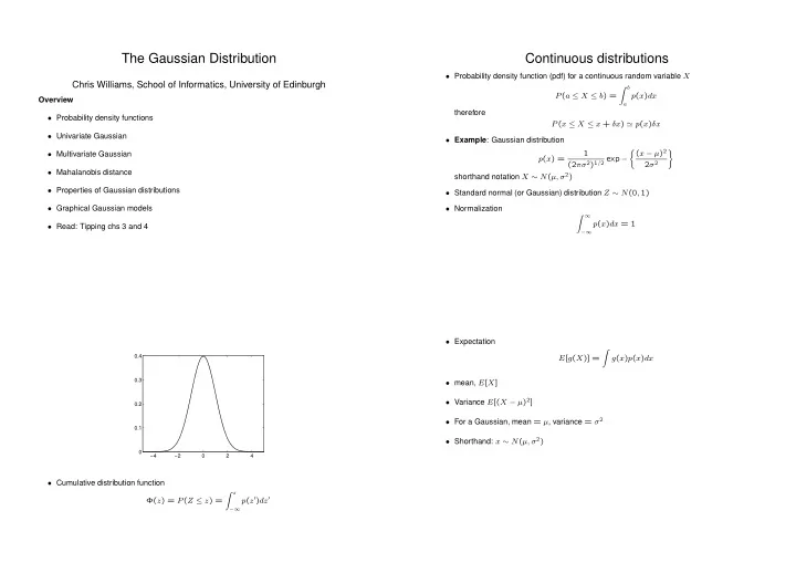
−4 −2 2 4 0.1 0.2 0.3 0.4

• Cumulative distribution function

Φ(z) = P(Z ≤ z) = z

−∞

p(z′)dz′

• Expectation

E[g(X)] =

• g(x)p(x)dx
• mean, E[X]
• Variance E[(X − µ)2]
• For a Gaussian, mean = µ, variance = σ2
• Shorthand: x ∼ N(µ, σ2)

Bivariate Gaussian I

• Let X1 ∼ N(µ1, σ2

1) and X2 ∼ N(µ2, σ2 2)

• If X1 and X2 are independent

p(x1, x2) = 1 2π(σ2

1σ2 2)1/2 exp −1

2 (x1 − µ1)2 σ2

1

+ (x2 − µ2)2 σ2

2

• Let x =
• x1

x2

• , µ =
• µ1

µ2

• , Σ =
• σ2

1

σ2

2

• p(x) =

1 2π|Σ|1/2 exp −1 2

• (x − µ)TΣ−1(x − µ)
• −2

−1 1 2 −2 −1 1 2 0.2 0.4 0.6 0.8 1

Bivariate Gaussian II

• Covariance
• Σ is the covariance matrix

Σ = E[(x − µ)(x − µ)T] Σij = E[(xi − µi)(xj − µj)]

• Example:

plot of weight vs height for a population

Multivariate Gaussian

• P(x ∈ R) =
• R p(x)dx
• Multivariate Gaussian

p(x) = 1 (2π)d/2|Σ|1/2 exp

• −1

2(x − µ)TΣ−1(x − µ)

• Σ is the covariance matrix

Σ = E[(x − µ)(x − µ)T] Σij = E[(xi − µi)(xj − µj)]

• Σ is symmetric
• Shorthand x ∼ N(µ, Σ)
• For p(x) to be a density, Σ must be positive definite
• Σ has d(d + 1)/2 parameters, the mean has a further d

Mahalanobis Distance

d2

Σ(xi, xj) = (xi − xj)TΣ−1(xi − xj)

• d2

Σ(xi, xj) is called the Mahalanobis distance between xi and xj

• If Σ is diagonal, the contours of d2

Σ are axis-aligned ellipsoids

• If Σ is not diagonal, the contours of d2

Σ are rotated ellipsoids

Σ = UΛU T where Λ is diagonal and U is a rotation matrix

• Σ is positive definite ⇒ entries in Λ are positive

Parameterization of the covariance matrix

• Fully general Σ =

⇒ variables are correlated

• Spherical or isotropic. Σ = σ2I. Variables are independent
• Diagonal [Σ]ij = δijσ2

i Variables are independent

• Rank-constrained: Σ = WW T + Ψ, with W being a d × q matrix with

q < d − 1 and Ψ diagonal. This is the factor analysis model. If Ψ = σ2I, then with have the probabilistic principal components analysis (PPCA) model

Transformations of Gaussian variables

• Linear transformations of Gaussian RVs are Gaussian

X ∼ N(µx, Σ) Y = AX + b Y ∼ N(Aµx + b, AΣAT)

• Sums of Gaussian RVs are Gaussian

Z = X + Y E[Z] = E[X] + E[Y ] var[Z] = var[X] + var[Y ] + 2covar[XY ] if X and Y are independent var[Z] = var[X] + var[Y ]

Properties of the Gaussian distribution

• Gaussian has relatively simple analytical properties
• Central limit theorem. Sum (or mean) of M independent random variables is distributed

normally as M → ∞ (subject to a few general conditions)

• Diagonalization of covariance matrix =

⇒ rotated variables are independent

• All marginal and conditional densities of a Gaussian are Gaussian
• The Gaussian is the distribution that maximizes the entropy H = −

p(x) log p(x)dx for fixed mean and covariance

Graphical Gaussian Models

Example:

x y z

• Let X denote pulse rate
• Let Y denote measurement taken by machine 1, and Z denote measurement taken by

machine 2

• Model

X ∼ N(µx, vx) Y = µy + wy(X − µx) + Ny Z = µz + wz(X − µx) + Nz noise Ny ∼ N(0, vN

y ), Nz ∼ N(0, vN z ), independent

• (X, Y, Z) is jointly Gaussian; can do inference for X given Y = y and Z = z

As before P(x, y, z) = P(x)P(y|x)P(z|x) Show that µ =

  

µx µy µz

  

Σ =

  

vx wyvx wzvx wyvx w2

yvx + vN y

wywzvx wzvx wywzvx w2

z vx + vN z   

Inference in Gaussian models

• Partition variables into two groups, X1 and X2

µ =

• µ1

µ2

• Σ =
• Σ11

Σ12 Σ21 Σ22

• µc

1|2 = µ1 + Σ12Σ−1 22 (x2 − µ2)

Σc

1|2 = Σ11 − Σ12Σ−1 22 Σ21

• For proof see §13.4 of Jordan (not examinable)
• Formation of joint Gaussian is analogous to formation of joint probability table for

discrete RVs. Propagation schemes are also possible for Gaussian RVs

Hybrid (discrete + continuous) networks

• Could discretize continuous variables, but this is ugly, and gives large

CPTs

• Better to use parametric families, e.g. Gaussian
• Works easily when continuous nodes are children of discrete nodes; we

then obtain a conditional Gaussian model