
SLIDE 1
ST 516 Experimental Statistics for Engineers II
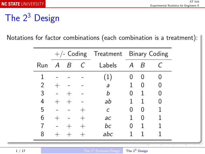
The 23 Design
Notations for factor combinations (each combination is a treatment): +/- Coding Treatment Binary Coding Run A B C Labels A B C 1
- (1)
2 +
- a
1 3
- +
- b
1 4 + +
- ab
1 1 5
- +
c 1 6 +
- +
ac 1 1 7
- +
+ bc 1 1 8 + + + abc 1 1 1
1 / 17 The 2k Factorial Design The 23 Design