Table of contents Inference of high-dimensional VAR models Linear - - PDF document

SLIDE 1

Inference of high-dimensional VAR models

Seminar: ”Modeling, Simulation and Inference of Complex Biological Systems” Katharina Schneider 07.07.2006

Linear time series Structural analysis with VAR models Estimation of VAR models Numerical examples

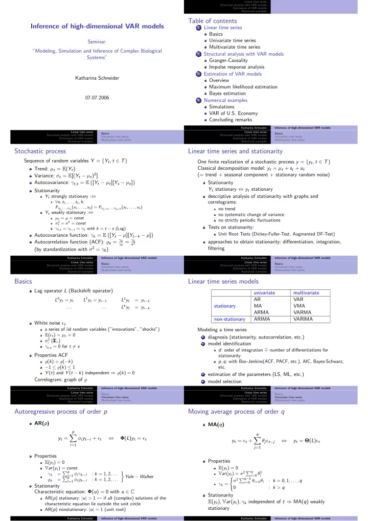
Table of contents

1

Linear time series Basics Univariate time series Multivariate time series

2

Structural analysis with VAR models Granger-Causality Impulse response analysis

3

Estimation of VAR models Overview Maximum likelihood estimation Bayes estimation

4

Numerical examples Simulations VAR of U.S. Economy Concluding remarks

Katharina Schneider Inference of high-dimensional VAR models Linear time series Structural analysis with VAR models Estimation of VAR models Numerical examples Basics Univariate time series Multivariate time series

Stochastic process

Sequence of random variables Y = {Yt, t ∈ T} Trend: µt = E(Yt) Variance: σt = E[(Yt − µt)2] Autocovariance: γt,s = E {[Yt − µt][Ys − µs]} Stationarity

Yt strongly stationary :⇔

∀n, t1, . . . , tn, h: Fxt1 ,...,xtn (x1, . . . , xn) = Fxt1+h,...,xtn+h(x1, . . . , xn)

Yt weakly stationary :⇔

µt = µ = const σ2

t = σ2 = const

γt,s = γt−s = γk with k = t − s (Lag)

Autocovariance function: γk = E {[Yt − µ][Yt−k − µ]} Autocorrelation function (ACF): ̺k = γk

γ0 = γk σ2

(by standardization with σ2 = γ0)

Katharina Schneider Inference of high-dimensional VAR models Linear time series Structural analysis with VAR models Estimation of VAR models Numerical examples Basics Univariate time series Multivariate time series

Linear time series and stationarity

One finite realization of a stochastic process y = {yt, t ∈ T} Classical decomposition model: yt = µt + st + ut (= trend + seasonal component + stationary random noise) Stationarity Yt stationary ⇔ yt stationary descriptive analysis of stationarity with graphs and correlograms:

no trend no systematic change of variance no strictly periodic fluctuations

Tests on stationarity:

Unit Root Tests (Dickey-Fuller-Test, Augmented DF-Test)

approaches to obtain stationarity: differentiation, integration, filtering

Katharina Schneider Inference of high-dimensional VAR models Linear time series Structural analysis with VAR models Estimation of VAR models Numerical examples Basics Univariate time series Multivariate time series

Basics

Lag operator L (Backshift operator)

L0yt = yt L1yt = yt−1 L2yt = yt−2 . . . . . . Lkyt = yt−k

White noise ǫt

a series of iid random variables (”innovations”, ”shocks”) E(ǫt) = µt = 0 σ2

ǫ (Σǫ)

γt,s = 0 for t = s

Properties ACF

̺(k) = ̺(−k) −1 ≤ ̺(k) ≤ 1 Y (t) and Y (t − k) independent ⇒ ̺(k) = 0

Correlogram: graph of ̺

Katharina Schneider Inference of high-dimensional VAR models Linear time series Structural analysis with VAR models Estimation of VAR models Numerical examples Basics Univariate time series Multivariate time series

Linear time series models

univariate multivariate AR VAR stationary MA VMA ARMA VARMA non-stationary ARIMA VARIMA Modeling a time series

1 diagnosis (stationarity, autocorrelation, etc.) 2 model identification

d: order of integration = number of differentiations for stationarity p, q: with Box-Jenkins(ACF, PACF, etc.), AIC, Bayes-Schwarz, etc.

3 estimation of the parameters (LS, ML, etc.) 4 model selection Katharina Schneider Inference of high-dimensional VAR models Linear time series Structural analysis with VAR models Estimation of VAR models Numerical examples Basics Univariate time series Multivariate time series

Autoregressive process of order p

AR(p) yt =

p

• i=1

φiyt−i + ǫt ⇔ Φ(L)yt = ǫt Properties

E(yt) = 0 Var(yt) = const. γk = p

l=1 φlγk−l

: k = 1, 2, . . . ̺k = p

l=1 φl̺k−l

: k = 1, 2, . . .

• Yule − Walker

Stationarity Characteristic equation: Φ(u) = 0 with u ∈ C

AR(p) stationary: |u| > 1 ↔ if all (complex) solutions of the characteristic equation lie outside the unit circle AR(p) nonstationary: |u| = 1 (unit root)

Katharina Schneider Inference of high-dimensional VAR models Linear time series Structural analysis with VAR models Estimation of VAR models Numerical examples Basics Univariate time series Multivariate time series

Moving average process of order q

MA(q) yt = ǫt +

q

• j=1

θjǫt−j ⇔ yt = Θ(L)ǫt Properties

E(yt) = 0 Var(yt) = σ2 q

i=0 θ2 i

γk =

• σ2 q−k

i=0 θi+kθi

: k = 0, 1, . . . , q : k > q

Stationarity E(yt), Var(yt), γk independent of t ⇒ MA(q) weakly stationary

Katharina Schneider Inference of high-dimensional VAR models

SLIDE 2

Linear time series Structural analysis with VAR models Estimation of VAR models Numerical examples Basics Univariate time series Multivariate time series

Autoregressive moving average process

ARMA(p, q) yt =

p

• i=1

φiyt−i + ǫt +

q

• j=1

θjǫt−j ⇔ Φ(L)yt = Θ(L)ǫt

Stationarity ARMA(p, q) stationary ⇔ AR(p)-part stationary

ARIMA(p, d, q) Autoregressive Integrated Moving Average Process Φ(L)(1 − L)dyt = Θ(L)ǫt ⇔ if xt := (1 − L)dyt ARMA(p, q)→{yt} ARIMA(p, d, q)

Stationarity ARIMA(p, d, q) stationary ⇔ d = 0 (i.e. ARMA(p, q))

Katharina Schneider Inference of high-dimensional VAR models Linear time series Structural analysis with VAR models Estimation of VAR models Numerical examples Basics Univariate time series Multivariate time series

Vector autoregressive model of order p

VAR(p) y′

t = c + L

• i=1

y′

t−iBi + ǫ′ t

for t = 1, . . . , T with yt (1 × p) random vector c unknown fixed (1 × p) vector of intercept terms Bi unknown fixed (p × p) regression coefficient matrices ǫt p-dimensional white noise process (ǫt ∼ iid(0, Σ)) L known positive integer (number of lags) t time period variable

Katharina Schneider Inference of high-dimensional VAR models Linear time series Structural analysis with VAR models Estimation of VAR models Numerical examples Basics Univariate time series Multivariate time series

Vector autoregressive model of order p

VAR(p) Y = XΦ + ǫ =      x′

1

: . . . x′

T

    

• T×(1+Lp)

     c B1 . . . BL     

• (1+Lp)×p

+      ǫ′

1

: . . . ǫ′

T

    

• T×p

=      y′

1

: . . . y′

T

    

• T×p

with xt =      1 y′

t−1

. . . y′

t−L

    

• (1+Lp)×1

ǫt ∼ iid(0, Σ) Σ := E(ǫtǫ′

t) = Cov(ǫt)

: positive definite p × p matrix

Katharina Schneider Inference of high-dimensional VAR models Linear time series Structural analysis with VAR models Estimation of VAR models Numerical examples Basics Univariate time series Multivariate time series

Vector autoregressive model of order p

Stability VAR(p) stable ⇔ det(I − Bu) = 0 for |u| ≤ 1 Stationarity VAR(p) stable ⇒ VAR(p) stationary L = 1 (VARs with one lag):

VAR(p) stationary ⇔ the absolute values of the real eigenvalues of B1 are less than unity VAR(p) nonstationary ⇔ the absolute values of the real eigenvalues of B1 lie on the unit circle

L > 1 (VARs with more than one lag): ⇒ rewrite as a VAR with one lag ⇒ stationarity is necessary for impulse response analysis and for estimation ⇒ problem: differentiation sometimes falsification

Katharina Schneider Inference of high-dimensional VAR models Linear time series Structural analysis with VAR models Estimation of VAR models Numerical examples Basics Univariate time series Multivariate time series

Moving average representation of a VAR(p)

y′

t = E0y′ t + t−1

• j=0

ǫ′

t−jHj

with VAR stationary H0 (p × p) identity matrix Hj impulse responses to a shock occuring j periods ago ⇒ yt is expressed in terms of past and present error/innovation vectors ǫt and the mean term ⇒ necessary for impulse response analysis ⇒ can be used to determine the autocovariances

Katharina Schneider Inference of high-dimensional VAR models Linear time series Structural analysis with VAR models Estimation of VAR models Numerical examples Granger-Causality Impulse response analysis

Characterization and interpretation of VARs

Characteristics VAR models are popular tools for analyzing multivariate time series data VAR models represent the correlations among a set of variables ⇒ analysis of certain aspects of the relationships between the interesting variables Structural analysis Granger-Causality impulse response analysis

Katharina Schneider Inference of high-dimensional VAR models Linear time series Structural analysis with VAR models Estimation of VAR models Numerical examples Granger-Causality Impulse response analysis

Granger-Causality

based on the principle of cause and effect MA representation of a K− dimensional VAR yt = µ + H(L)ǫt with H0 = IK partitioned MA representation yt = zt xt

• =

µ1 µ2

• +

H11(L) H12(L) H21(L) H22(L) ǫ1t ǫ2t

• with

zt M-dimensional xt (K − M)-dimensional ⇒zt is not Granger-caused by xt :⇔ H12,i = 0 for i = 1, 2, . . . xt is Granger-causal to zt ⇔ the information in the past and the present of x helps to predict zt+1

Katharina Schneider Inference of high-dimensional VAR models Linear time series Structural analysis with VAR models Estimation of VAR models Numerical examples Granger-Causality Impulse response analysis

Impulse response functions

MA representation y′

t = E0y′ t + t−1

• j=0

ǫ′

t−jHj

impulse responses of yt to a shock ǫt−j occuring j periods earlier Hj =

j

• i=1

BiHj−i with Bi = 0 for i > L ǫt correlated

Katharina Schneider Inference of high-dimensional VAR models

SLIDE 3

Linear time series Structural analysis with VAR models Estimation of VAR models Numerical examples Granger-Causality Impulse response analysis

Problem: ǫt are correlated → identification problem Solution: orthogonalization of the errors Cholesky decomposition of the covariance matrix Σ = Ψ′Ψ with Ψ uppertriangular positive definite matrix connection between structural shocks and VAR errors u′

t = ǫ′ tΨ−1

with ut structural error vector (with Σ(ut): identity matrix) impulse responses to structural shocks occuring j periods earlier Zj = ΨHj

Katharina Schneider Inference of high-dimensional VAR models Linear time series Structural analysis with VAR models Estimation of VAR models Numerical examples Overview Maximum likelihood estimation Bayes estimation

Possibilities for estimating a VAR

Least Squares ⇒ asymptotic properties Maximum Likelihood ⇒ assumption: known distribution of data ⇒ for some distributions MLE does not have an analytical form or does not exist Bayes ⇒ effectiveness for finite-sample inference ⇒ the estimated process may be used for prediction and economic analyses ⇒ applicable to estimate the model parameters and to estimate the distributions of the impulse response functions

Katharina Schneider Inference of high-dimensional VAR models Linear time series Structural analysis with VAR models Estimation of VAR models Numerical examples Overview Maximum likelihood estimation Bayes estimation

MLE for normal VARs

Y = XΦ + ǫ ǫ iid ∼ Np(0, Σ) Likelihood function of (Φ, Σ) lN(Φ, Σ) = 1 |Σ|T/2 exp

• −1

2

T

• t=1

(yt − xtΦ)′Σ−1(yt − xtΦ)

• =

1 |Σ|T/2 etr

• =exp(trace)
• −1

2(Y − XΦ)Σ−1(Y − XΦ)′

• Maximum likelihood estimators (MLEs)
• ΦMLE

= (X′X)−1X′Y

• ΣMLE

= S( ΦMLE) T with S(Φ) = (Y − XΦ)′(Y − XΦ)

Katharina Schneider Inference of high-dimensional VAR models Linear time series Structural analysis with VAR models Estimation of VAR models Numerical examples Overview Maximum likelihood estimation Bayes estimation

MLE for Student-t VARs

Y = XΦ + ǫ ǫt

ind.

∼ tν(0, Σ) Density of tν(0, Σ) (multivariate-t distribution) p (s|Σ, ν) = Γ 1

2(ν + p)

• (πν)p/2 Γ(ν

2) × |Σ|−1/2

• 1 + 1

ν s′ Σ−1s −(p+ν)

2

, s ∈ Rp Maximum likelihood estimators (MLEs)

ν given ⇒ MLE for (Φ, Σ) is not available in closed form ν unknown ⇒ MLE for (Φ, Σ, ν) may not even exist

Katharina Schneider Inference of high-dimensional VAR models Linear time series Structural analysis with VAR models Estimation of VAR models Numerical examples Overview Maximum likelihood estimation Bayes estimation

Basics

A Bayesian estimator of (Φ, Σ) depends on the distribution model the prior the loss function Bayesian procedure

1 choose a prior 2 derive/compute the posterior 3 choose a loss function 4 estimate under the loss function 5 calculate the risk function 6 evaluate the performance of the estimates Katharina Schneider Inference of high-dimensional VAR models Linear time series Structural analysis with VAR models Estimation of VAR models Numerical examples Overview Maximum likelihood estimation Bayes estimation

Priors for φ, Σ

PPPPPPPP P

for φ for Σ Jeffreys prior RATS prior Reference prior Constant prior πCJ(φ, Σ) πCA(φ, Σ) πCR(φ, Σ) Shrinkage prior πSJ(φ, Σ) πSA(φ, Σ) πSR(φ, Σ) ⇒ noninformative priors Prior for ν in the Student-t VAR w = ν 2 with w ∼ Gamma(a, b) a, b known positive constants

Katharina Schneider Inference of high-dimensional VAR models Linear time series Structural analysis with VAR models Estimation of VAR models Numerical examples Overview Maximum likelihood estimation Bayes estimation

Jeffreys prior

Jeffreys prior for the normal VAR model Jeffreys prior for Σ: πJ(Σ) ∝ |Σ|−(p+1)/2 constant Jeffreys prior for (Φ, Σ): πCJ(φ, Σ) ∝ πJ(Σ)

conditional posterior of φ given (Σ, Y): NJ( φMLE, Σ ⊗ (X′X)−1) marginal posterior of Σ given Y: Inverse Wishart(S( ΦMLE), T − Lp − 1)

⇒ derived from the ”invariance principle” Shrinkage Jeffreys prior for (Φ, Σ): πSJ(φ, Σ) = πS(φ)πJ(Σ) ⇒ motivated by Stein´s result on inadmissibility of the MLE

Katharina Schneider Inference of high-dimensional VAR models Linear time series Structural analysis with VAR models Estimation of VAR models Numerical examples Overview Maximum likelihood estimation Bayes estimation

Loss functions for Σ

1 pseudoentropy loss

LΣ1( Σ; Σ) = trace( Σ

−1Σ) − log|

Σ

−1Σ| − p

2 quadratic loss

LΣ2( Σ; Σ) = trace( ΣΣ−1 − I)2

3 pseudoentropy function on Σ−1

LΣ3( Σ; Σ) = trace( ΣΣ−1) − log| ΣΣ−1| − p

Katharina Schneider Inference of high-dimensional VAR models

SLIDE 4

Linear time series Structural analysis with VAR models Estimation of VAR models Numerical examples Overview Maximum likelihood estimation Bayes estimation

Loss functions for Φ

1 quadratic loss

LΦ1( Φ, Φ) = trace

• (

Φ − Φ)′ W ( Φ − Φ)

• with

W constant weighting matrix here: W = I ⇒ LΦ1 =

1+Lp

• i=1

p

• j=1

( φij − φij)2 → symmetric

2 LINEX loss

LΦ2( Φ, Φ) =

1+Lp

• i=1

p

• j=1
• exp
• aij(

φij − φij)

• − aij(

φij − φij) − 1

• with aij

given constant → asymmetric

Katharina Schneider Inference of high-dimensional VAR models Linear time series Structural analysis with VAR models Estimation of VAR models Numerical examples Overview Maximum likelihood estimation Bayes estimation

Loss and risk function for impulse response functions

Loss function L(Zj, Zj) = trace

• (Zj −

Zj)′ Ω (Zj − Zj)

• with Ω: weighting matrix for the estimation error of each element
• f the impulse responses

→ may be determined by the economic significance of the element (here: identity matrix) Risk function RImp,i = 1 N

N

• n=1

trace

• Zi −

Z

(n) i

′ −

• Zi −

Z

(n) i

• with

Z

(n) i

: impulse response matrix for the ith step after the shock for the nth dataset generated in the experiment

Katharina Schneider Inference of high-dimensional VAR models Linear time series Structural analysis with VAR models Estimation of VAR models Numerical examples Simulations VAR of U.S. Economy Concluding remarks

Simulations and Bayesian computation

1 generate N = 1, 000 data samples from a VAR(5) model with

• ne lag (L = 1) and the known parameters

Σ = ✵ ❇ ❇ ❅ 1.0 0.5 ... 0.5 1.0 ✶ ❈ ❈ ❆ , Φ = ✒ c B1 ✓ = ✒ I5 ✓ , ν = 8 prior for ν : ν ∼ Gamma(1, 0.5) 2 compute the Bayesian estimates under competing priors and

the different losses via MCMC (M = 10, 000 cycles)

1

find the full conditional distributions of (φ, Σ) with φ = vec(Φ)

2

simulate the posteriors of (Φ, Σ)

3 estimate the frequentist risks under a loss L of the estimates

as the average loss belonging to Σ and Φ across generated data samples

4 evaluate the performance of the Bayesian estimates in terms

• f the frequentist risks given the true parameters

Katharina Schneider Inference of high-dimensional VAR models Linear time series Structural analysis with VAR models Estimation of VAR models Numerical examples Simulations VAR of U.S. Economy Concluding remarks

Frequentist average losses of competing Bayes estimates of Σ in the normal VAR

Katharina Schneider Inference of high-dimensional VAR models Linear time series Structural analysis with VAR models Estimation of VAR models Numerical examples Simulations VAR of U.S. Economy Concluding remarks

Frequentist average losses of competing Bayes estimates of Σ in the normal VAR

Katharina Schneider Inference of high-dimensional VAR models Linear time series Structural analysis with VAR models Estimation of VAR models Numerical examples Simulations VAR of U.S. Economy Concluding remarks

Frequentist average losses of competing Bayes estimates of Φ in the normal VAR

Katharina Schneider Inference of high-dimensional VAR models Linear time series Structural analysis with VAR models Estimation of VAR models Numerical examples Simulations VAR of U.S. Economy Concluding remarks

Frequentist average losses of competing Bayes estimates of Φ in the normal VAR

Katharina Schneider Inference of high-dimensional VAR models Linear time series Structural analysis with VAR models Estimation of VAR models Numerical examples Simulations VAR of U.S. Economy Concluding remarks

Estimation of impulse response functions

Zj are nonlinear functions of (Φ, Σ)⇒ Bayes-simulations

1 generate data samples from a VAR with known parameters 2 compute the Bayesian estimates under competing priors via

MCMC

1

find the full conditional distributions of (Z)

2

simulate the posteriors of (Z)

3

compute Zj = E(Zj| Y) (assumption: Ω const.)

3 evaluate the performance of the estimates in terms of the

frequentist average of sum of squared errors

Katharina Schneider Inference of high-dimensional VAR models

SLIDE 5

Linear time series Structural analysis with VAR models Estimation of VAR models Numerical examples Simulations VAR of U.S. Economy Concluding remarks

Frequentist average losses of impulse responses in the normal VAR

Katharina Schneider Inference of high-dimensional VAR models Linear time series Structural analysis with VAR models Estimation of VAR models Numerical examples Simulations VAR of U.S. Economy Concluding remarks

Frequentist average losses of impulse responses in the Student-t VAR

Katharina Schneider Inference of high-dimensional VAR models Linear time series Structural analysis with VAR models Estimation of VAR models Numerical examples Simulations VAR of U.S. Economy Concluding remarks

VAR of U.S. Economy

VAR(6) model with two lags (L=2) quarterly data of the U.S. economy from 1959 Q1 to 2001 Q4

real GDP(Gross Domestic Product) GDP deflator world commodity price Federal Funds rates nonborrowed reserves M2 money stock

M = 10, 000 MCMC cycles

Katharina Schneider Inference of high-dimensional VAR models Linear time series Structural analysis with VAR models Estimation of VAR models Numerical examples Simulations VAR of U.S. Economy Concluding remarks

Responses of GDP to an inflation shock

constant RATS prior constant Jeffreys prior constant reference prior shrinkage RATS prior shrinkage Jeffreys prior shrinkage reference prior

Katharina Schneider Inference of high-dimensional VAR models Linear time series Structural analysis with VAR models Estimation of VAR models Numerical examples Simulations VAR of U.S. Economy Concluding remarks

Concluding remarks

Simulations → the choice of prior has stronger effects on the Bayesian estimates than the choice of loss function → the asymmetric LINEX estimator for Φ does better overall than the posterior mean → there is no estimator for Σ dominating in all cases → the shrinkage prior dominates the constant prior → reference prior on Σ dominates the Jeffreys prior and the RATS prior

Katharina Schneider Inference of high-dimensional VAR models Linear time series Structural analysis with VAR models Estimation of VAR models Numerical examples Simulations VAR of U.S. Economy Concluding remarks

Concluding remarks

VAR of U.S. Economy → significant improvement of the estimates by using alternative priors in place of constant prior → impulse responses of GDP to an inflation shock are distinctly different under the competing priors → the posterior losses under the shrinkage reference prior are smaller → VAR model estimates allow some degree of collinearity and have no restrictions on the matrix Φ → MLEs are often very sensitive to model specification and sample period

Katharina Schneider Inference of high-dimensional VAR models Linear time series Structural analysis with VAR models Estimation of VAR models Numerical examples Simulations VAR of U.S. Economy Concluding remarks

Literature

NI, S. & SUN, D. (2005): Bayesian Estimates for Vector Autoregressive Models. Journal of Business & Economic Statistics, 23: 105–117. L¨ UTKEPOHL, H. (1993): Introduction to Multiple Time Series Analysis. Springer Verlag, Berlin, Heidelberg. BROCKWELL, P.J. & DAVIS, R.A. (1996): Introduction to Time Series and Forecasting. Springer Verlag, New York. MANSMANN, U. (2006): Skript zur Vorlesung Zeitreihenanalyse.

Katharina Schneider Inference of high-dimensional VAR models