Stereo Thurs Mar 23 Kristen Grauman UT Austin Previously Write - - PDF document

3/22/2017 1

Thurs Mar 23 Kristen Grauman UT Austin

Stereo Previously

• Write 2d transformations as matrix-vector

multiplication

• Perform image warping (forward, inverse)
• Fitting transformations: solve for unknown

parameters given corresponding points from two views (affine, projective (homography)).

• Mosaics: uses homography and image warping

to merge views taken from same center of projection.

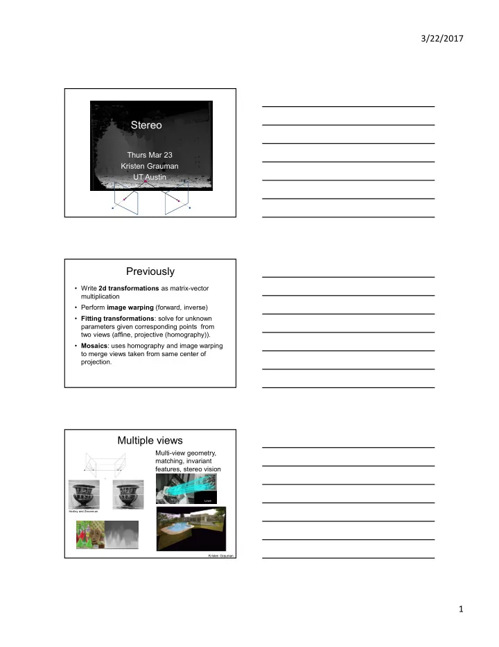
Multiple views

Hartley and Zisserman Lowe

Multi-view geometry, matching, invariant features, stereo vision

Kristen Grauman

3/22/2017 2 Why multiple views?

• Structure and depth are inherently ambiguous from

single views.

Images from Lana Lazebnik

Why multiple views?

• Structure and depth are inherently ambiguous from

single views.

Optical center

P1 P2 P1’=P2’

Kristen Grauman

• What cues help us to perceive 3d shape

and depth?

3/22/2017 3

Texture

[From A.M. Loh. The recovery of 3-D structure using visual texture patterns. PhD thesis]

Perspective effects

Image credit: S. Seitz

Shading

[Figure from Prados & Faugeras 2006]

3/22/2017 4

Focus/defocus

[figs from H. Jin and P. Favaro, 2002]

Images from same point of view, different camera parameters 3d shape / depth estimates

Motion

Figures from L. Zhang http://www.brainconnection.com/teasers/?main=illusion/motion-shape

Estimating scene shape

• “Shape from X”: Shading, Texture, Focus, Motion…
• Stereo:

– shape from “motion” between two views – infer 3d shape of scene from two (multiple) images from different viewpoints

scene point

• ptical center

image plane

Main idea:

Kristen Grauman

3/22/2017 5

Outline

• Human stereopsis
• Epipolar geometry and the epipolar constraint

– Case example with parallel optical axes – General case with calibrated cameras

• Stereo solutions

– Correspondences – Additional constraints

Human eye

Fig from Shapiro and Stockman

Pupil/Iris – control amount of light passing through lens Retina - contains sensor cells, where image is formed Fovea – highest concentration of cones

Human stereopsis: disparity

Human eyes fixate on point in space – rotate so that corresponding images form in centers of fovea.

3/22/2017 6

Disparity occurs when eyes fixate on one object;

• thers appear at different

visual angles

Human stereopsis: disparity

Disparity: d = r-l = D-F. d=0

Human stereopsis: disparity

Forsyth & Ponce

Random dot stereograms

• Julesz 1960: Do we identify local brightness

patterns before fusion (monocular process) or after (binocular)?

• To test: pair of synthetic images obtained by

randomly spraying black dots on white objects

3/22/2017 7

Random dot stereograms

Forsyth & Ponce

Random dot stereograms Random dot stereograms

• When viewed monocularly, they appear random;

when viewed stereoscopically, see 3d structure.

• Conclusion: human binocular fusion not directly

associated with the physical retinas; must involve the central nervous system

• Imaginary “cyclopean retina” that combines the

left and right image stimuli as a single unit

3/22/2017 8 Stereo photography and stereo viewers

Invented by Sir Charles Wheatstone, 1838

Image from fisher-price.com

Take two pictures of the same subject from two slightly different viewpoints and display so that each eye sees

• nly one of the images.

http://www.johnsonshawmuseum.org http://www.johnsonshawmuseum.org

3/22/2017 9

Public Library, Stereoscopic Looking Room, Chicago, by Phillips, 1923

http://www.well.com/~jimg/stereo/stereo_list.html

Kristen Grauman

Autostereograms

Images from magiceye.com

Exploit disparity as depth cue using single image. (Single image random dot stereogram, Single image stereogram)

Kristen Grauman

3/22/2017 10

Images from magiceye.com

Autostereograms

Kristen Grauman

Camera parameters

Camera frame 1

Intrinsic parameters: Image coordinates relative to camera  Pixel coordinates Extrinsic parameters: Camera frame 1  Camera frame 2

Camera frame 2

• Extrinsic params: rotation matrix and translation vector
• Intrinsic params: focal length, pixel sizes (mm), image center

point, radial distortion parameters

We’ll assume for now that these parameters are given and fixed.

Outline

• Human stereopsis
• Stereograms
• Epipolar geometry and the epipolar constraint

– Case example with parallel optical axes – General case with calibrated cameras

3/22/2017 11

Two cameras, simultaneous views Single moving camera and static scene

Stereo vision

Kristen Grauman

Estimating depth with stereo

• Stereo: shape from “motion” between two views
• We’ll need to consider:
• Info on camera pose (“calibration”)
• Image point correspondences

scene point

• ptical

center image plane

Geometry for a simple stereo system

• First, assuming parallel optical axes, known camera

parameters (i.e., calibrated cameras):

3/22/2017 12

baseline

• ptical

center (left)

• ptical

center (right) Focal length World point image point (left) image point (right) Depth of p

• Assume parallel optical axes, known camera parameters

(i.e., calibrated cameras). What is expression for Z? Similar triangles (pl, P, pr) and (Ol, P, Or):

Geometry for a simple stereo system

Z T f Z x x T

r l

   

l r

x x T f Z  

disparity

Depth from disparity

image I(x,y) image I´(x´,y´) Disparity map D(x,y)

(x´,y´)=(x+D(x,y), y) So if we could find the corresponding points in two images, we could estimate relative depth…

3/22/2017 13

Outline

• Human stereopsis
• Stereograms
• Epipolar geometry and the epipolar constraint

– Case example with parallel optical axes – General case with calibrated cameras

General case, with calibrated cameras

• The two cameras need not have parallel optical axes.

Vs.

• Given p in left image, where can corresponding

point p’ be?

Stereo correspondence constraints

3/22/2017 14

Stereo correspondence constraints

Geometry of two views constrains where the corresponding pixel for some image point in the first view must occur in the second view.

• It must be on the line carved out by a plane

connecting the world point and optical centers.

Epipolar constraint

• Epipolar Plane

Epipole Epipolar Line Baseline

Epipolar geometry

Epipole http://www.ai.sri.com/~luong/research/Meta3DViewer/EpipolarGeo.html

3/22/2017 15

• Baseline: line joining the camera centers
• Epipole: point of intersection of baseline with image plane
• Epipolar plane: plane containing baseline and world point
• Epipolar line: intersection of epipolar plane with the image

plane

• All epipolar lines intersect at the epipole
• An epipolar plane intersects the left and right image planes

in epipolar lines

Epipolar geometry: terms

Why is the epipolar constraint useful?

Epipolar constraint

This is useful because it reduces the correspondence problem to a 1D search along an epipolar line.

Image from Andrew Zisserman

Example

3/22/2017 16

What do the epipolar lines look like?

Ol Or Ol Or

1. 2.

Kristen Grauman

Example: converging cameras

Figure from Hartley & Zisserman Figure from Hartley & Zisserman

Example: parallel cameras

Where are the epipoles?

3/22/2017 17

Stereo image rectification

reproject image planes onto a common plane parallel to the line between optical centers pixel motion is horizontal after this transformation two homographies (3x3 transforms), one for each input image reprojection

Slide credit: Li Zhang

In practice, it is convenient if image scanlines (rows) are the epipolar lines.

Stereo image rectification: example

Source: Alyosha Efros

An audio camera & epipolar geometry

Adam O' Donovan, Ramani Duraiswami and Jan Neumann Microphone Arrays as Generalized Cameras for Integrated Audio Visual Processing, IEEE Conference on Computer Vision and Pattern Recognition (CVPR), Minneapolis, 2007

Spherical microphone array

3/22/2017 18

An audio camera & epipolar geometry An audio camera & epipolar geometry

Summary so far

• Depth from stereo: main idea is to triangulate

from corresponding image points.

• Epipolar geometry defined by two cameras

– We’ve assumed known extrinsic parameters relating their poses

• Epipolar constraint limits where points from one

view will be imaged in the other

– Makes search for correspondences quicker

• Terms: epipole, epipolar plane / lines, disparity,

rectification, baseline

3/22/2017 19

Correspondence problem

Multiple match hypotheses satisfy epipolar constraint, but which is correct?

Figure from Gee & Cipolla 1999

Correspondence problem

• Beyond the hard constraint of epipolar

geometry, there are “soft” constraints to help identify corresponding points

– Similarity – Uniqueness – Ordering – Disparity gradient

• To find matches in the image pair, we will

assume

– Most scene points visible from both views – Image regions for the matches are similar in appearance

Dense correspondence search

For each epipolar line For each pixel / window in the left image

• compare with every pixel / window on same epipolar line in right

image

• pick position with minimum match cost (e.g., SSD, correlation)

Adapted from Li Zhang

3/22/2017 20

Correspondence problem

Source: Andrew Zisserman

Parallel camera example: epipolar lines are corresponding image scanlines

Correspondence problem

Source: Andrew Zisserman

Intensity profiles

Correspondence problem

Neighborhoods of corresponding points are similar in intensity patterns.

Source: Andrew Zisserman

3/22/2017 21

Normalized cross correlation

Source: Andrew Zisserman

Correlation-based window matching

Source: Andrew Zisserman

Textureless regions

Textureless regions are non-distinct; high ambiguity for matches.

Source: Andrew Zisserman

3/22/2017 22

Effect of window size?

Source: Andrew Zisserman

W = 3 W = 20

Figures from Li Zhang

Want window large enough to have sufficient intensity variation, yet small enough to contain only pixels with about the same disparity.

Effect of window size Foreshortening effects

Source: Andrew Zisserman

3/22/2017 23

Occlusion

Slide credit: David Kriegman

Sparse correspondence search

• Restrict search to sparse set of detected features (e.g., corners)
• Rather than pixel values (or lists of pixel values) use feature

descriptor and an associated feature distance

• Still narrow search further by epipolar geometry

Tradeoffs between dense and sparse search?

Correspondence problem

• Beyond the hard constraint of epipolar

geometry, there are “soft” constraints to help identify corresponding points

– Similarity – Uniqueness – Disparity gradient – Ordering

3/22/2017 24

Uniqueness constraint

• Up to one match in right image for every point in left

image

Figure from Gee & Cipolla 1999

Disparity gradient constraint

• Assume piecewise continuous surface, so want disparity

estimates to be locally smooth

Figure from Gee & Cipolla 1999

Ordering constraint

• Points on same surface (opaque object) will be in same
• rder in both views

Figure from Gee & Cipolla 1999

3/22/2017 25

Ordering constraint

Figures from Forsyth & Ponce

• Won’t always hold, e.g. consider transparent object, or

an occluding surface

• Beyond individual correspondences to estimate

disparities:

• Optimize correspondence assignments jointly

– Scanline at a time (DP) – Full 2D grid (graph cuts)

Scanline stereo

• Try to coherently match pixels on the entire scanline
• Different scanlines are still optimized independently

Left image Right image

intensity

3/22/2017 26

“Shortest paths” for scan-line stereo

Left image Right image

Can be implemented with dynamic programming Ohta & Kanade ’85, Cox et al. ‘96

left

S

right

S

q p

Left

• cclusion

t

Right

• cclusion

s

I I

Slide credit: Y. Boykov

“Shortest paths” for scan-line stereo

Left image Right image

Can be implemented with dynamic programming Ohta & Kanade ’85, Cox et al. ‘96

left

S

right

S

I I

Slide credit: Y. Boykov

Coherent stereo on 2D grid

• Scanline stereo generates streaking artifacts
• Can’t use dynamic programming to find spatially

coherent disparities/ correspondences on a 2D grid

3/22/2017 27

Stereo matching as energy minimization

I1 I2 D W1(i) W2(i+D(i)) D(i)

) ( ) , , (

smooth 2 1 data

D E D I I E E      



 

j i

j D i D E

, neighbors smooth

) ( ) ( 

 

2 2 1 data

)) ( ( ) (



  

i

i D i W i W E

Stereo matching as energy minimization

I1 I2 D

• Energy functions of this form can be minimized using

graph cuts

Y . Boykov, O. Veksler, and R. Zabih, Fast Approximate Energy Minimization via Graph Cuts, PAMI 2001

W1(i) W2(i+D(i)) D(i)

) ( ) , , (

smooth 2 1 data

D E D I I E E      



 

j i

j D i D E

, neighbors smooth

) ( ) ( 

 

2 2 1 data

)) ( ( ) (



  

i

i D i W i W E

Source: Steve Seitz

Error sources

• Low-contrast ; textureless image regions
• Occlusions
• Camera calibration errors
• Violations of brightness constancy (e.g.,

specular reflections)

• Large motions

3/22/2017 28

Depth for segmentation

Danijela Markovic and Margrit Gelautz, Interactive Media Systems Group, Vienna University of Technology

Edges in disparity in conjunction with image edges enhances contours found

Depth for segmentation

Danijela Markovic and Margrit Gelautz, Interactive Media Systems Group, Vienna University of Technology

Model-based body tracking, stereo input

David Demirdjian, MIT Vision Interface Group http://people.csail.mit.edu/demirdji/movie/artic-tracker/turn-around.m1v

3/22/2017 29

Virtual viewpoint video

• C. Zitnick et al, High-quality video view interpolation using a layered representation,

SIGGRAPH 2004.

Virtual viewpoint video

http://research.microsoft.com/IVM/VVV/

• C. Larry Zitnick et al, High-quality video view interpolation using a layered

representation, SIGGRAPH 2004.

Summary

• Depth from stereo: main idea is to triangulate

from corresponding image points.

• Epipolar geometry defined by two cameras

– We’ve assumed known extrinsic parameters relating their poses

• Epipolar constraint limits where points from one

view will be imaged in the other

– Makes search for correspondences quicker

• To estimate depth

– Limit search by epipolar constraint – Compute correspondences, incorporate matching preferences

3/22/2017 30

Coming up

• Instance recognition

– Indexing local features efficiently – Spatial verification models