Today Recap: epipolar constraint Stereo image rectification - - PDF document

SLIDE 1

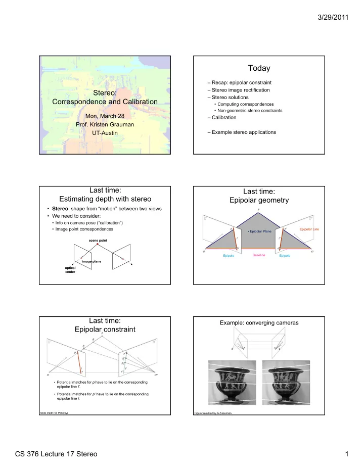
3/29/2011 CS 376 Lecture 17 Stereo 1 Stereo: Correspondence and Calibration

Mon, March 28

• Prof. Kristen Grauman

UT-Austin

Today

– Recap: epipolar constraint – Stereo image rectification – Stereo solutions

• Computing correspondences
• Non-geometric stereo constraints

– Calibration – Example stereo applications

Last time: Estimating depth with stereo

• Stereo: shape from “motion” between two views
• We need to consider:
• Info on camera pose (“calibration”)
• Image point correspondences

scene point

• ptical

center image plane

• Epipolar Plane

Epipole Epipolar Line Baseline

Last time: Epipolar geometry

Epipole

• Potential matches for p have to lie on the corresponding

epipolar line l’.

• Potential matches for p’ have to lie on the corresponding

epipolar line l.

Slide credit: M. Pollefeys

Last time: Epipolar constraint

Example: converging cameras

Figure from Hartley & Zisserman

SLIDE 2

3/29/2011 CS 376 Lecture 17 Stereo 2

Figure from Hartley & Zisserman

Example: parallel cameras

An audio camera & epipolar geometry

Adam O' Donovan, Ramani Duraiswami and Jan Neumann Microphone Arrays as Generalized Cameras for Integrated Audio Visual Processing, IEEE Conference on Computer Vision and Pattern Recognition (CVPR), Minneapolis, 2007

Spherical microphone array

An audio camera & epipolar geometry

Last time: Essential matrix

 

    RX T X

 

] [T    RX X

x

E is called the essential matrix, and it relates corresponding points between both cameras, given the rotation and translation. If we observe a point in one image, its position in other image is constrained to lie on line defined by above. Note: these points are in camera coordinate systems. Let

R E ] [T x    EX X T     



]R [ E T I R

x

T ] , , [ d

0 0 0 0 0 d 0 –d 0

 Ep p

Essential matrix example: parallel cameras

For the parallel cameras, image of any point must lie

• n same horizontal line in

each image plane.

] , ' , ' [ ] , , [ f y x f y x   p' p

image I(x,y) image I´(x´,y´) Disparity map D(x,y)

(x´,y´)=(x+D(x,y),y) What about when cameras’ optical axes are not parallel?

SLIDE 3

3/29/2011 CS 376 Lecture 17 Stereo 3

Today

– Recap: epipolar constraint – Stereo image rectification – Stereo solutions

• Computing correspondences
• Non-geometric stereo constraints

– Calibration – Example stereo applications

Stereo image rectification

reproject image planes onto a common plane parallel to the line between optical centers pixel motion is horizontal after this transformation two homographies (3x3 transforms), one for each input image reprojection

Slide credit: Li Zhang

In practice, it is convenient if image scanlines (rows) are the epipolar lines.

Stereo image rectification: example

Source: Alyosha Efros

Today

– Recap: epipolar constraint – Stereo image rectification – Stereo solutions

• Computing correspondences
• Non-geometric stereo constraints

– Calibration – Example stereo applications

Correspondence problem

Multiple match hypotheses satisfy epipolar constraint, but which is correct?

Figure from Gee & Cipolla 1999

Correspondence problem

• Beyond the hard constraint of epipolar

geometry, there are “soft” constraints to help identify corresponding points

– Similarity – Uniqueness – Ordering – Disparity gradient

• To find matches in the image pair, we will

assume

– Most scene points visible from both views – Image regions for the matches are similar in appearance

SLIDE 4

3/29/2011 CS 376 Lecture 17 Stereo 4

Dense correspondence search

For each epipolar line For each pixel / window in the left image

• compare with every pixel / window on same epipolar line in right

image

• pick position with minimum match cost (e.g., SSD, correlation)

Adapted from Li Zhang

Correspondence problem

Source: Andrew Zisserman

Parallel camera example: epipolar lines are corresponding image scanlines

Correspondence problem

Source: Andrew Zisserman

Intensity profiles

Correspondence problem

Neighborhoods of corresponding points are similar in intensity patterns.

Source: Andrew Zisserman

Correlation‐based window matching

Source: Andrew Zisserman

Textureless regions

Textureless regions are non‐distinct; high ambiguity for matches.

Source: Andrew Zisserman

SLIDE 5

3/29/2011 CS 376 Lecture 17 Stereo 5

Effect of window size

Source: Andrew Zisserman

W = 3 W = 20

Figures from Li Zhang

Want window large enough to have sufficient intensity variation, yet small enough to contain only pixels with about the same disparity.

Effect of window size Foreshortening effects

Source: Andrew Zisserman

Occlusion

Slide credit: David Kriegman

Sparse correspondence search

• Restrict search to sparse set of detected features (e.g., corners)
• Rather than pixel values (or lists of pixel values) use feature

descriptor and an associated feature distance

• Still narrow search further by epipolar geometry

Tradeoffs between dense and sparse search?

Correspondence problem

• Beyond the hard constraint of epipolar

geometry, there are “soft” constraints to help identify corresponding points

– Similarity – Uniqueness – Disparity gradient – Ordering

SLIDE 6

3/29/2011 CS 376 Lecture 17 Stereo 6

Uniqueness constraint

• Up to one match in right image for every point in left

image

Figure from Gee & Cipolla 1999

Disparity gradient constraint

• Assume piecewise continuous surface, so want disparity

estimates to be locally smooth

Figure from Gee & Cipolla 1999

Ordering constraint

• Points on same surface (opaque object) will be in same
• rder in both views

Figure from Gee & Cipolla 1999

Ordering constraint

Figures from Forsyth & Ponce

• Won’t always hold, e.g. consider transparent object, or

an occluding surface

• Beyond individual correspondences to estimate

disparities:

• Optimize correspondence assignments jointly

– Scanline at a time (DP) – Full 2D grid (graph cuts)

Scanline stereo

• Try to coherently match pixels on the entire scanline
• Different scanlines are still optimized independently

Left image Right image

intensity

SLIDE 7

3/29/2011 CS 376 Lecture 17 Stereo 7

“Shortest paths” for scan-line stereo

Left image Right image

Can be implemented with dynamic programming Ohta & Kanade ’85, Cox et al. ‘96

left

S

right

S

q p

Left

• cclusion

t

Right

• cclusion

s

I I

Slide credit: Y . Boykov

Coherent stereo on 2D grid

• Scanline stereo generates streaking artifacts
• Can’t use dynamic programming to find spatially

coherent disparities/ correspondences on a 2D grid

Stereo matching as energy minimization

I1 I2 D

• Energy functions of this form can be minimized using

graph cuts

• Y. Boykov, O. Veksler, and R. Zabih, Fast Approximate Energy Minimization

via Graph Cuts, PAMI 2001

W1(i) W2(i+D(i)) D(i)

) ( ) , , (

smooth 2 1 data

D E D I I E E      



 

j i

j D i D E

, neighbors smooth

) ( ) ( 

 

2 2 1 data

)) ( ( ) (



  

i

i D i W i W E

Source: Steve Seitz

Recap: stereo with calibrated cameras

• Given image pair, R, T
• Detect some features
• Compute essential matrix E
• Match features using the

epipolar and other constraints

• Triangulate for 3d structure

Error sources

• Low-contrast ; textureless image regions
• Occlusions
• Camera calibration errors
• Violations of brightness constancy (e.g.,

specular reflections)

• Large motions

Today

– Recap: epipolar constraint – Stereo image rectification – Stereo solutions

• Computing correspondences
• Non-geometric stereo constraints

– Calibration – Example stereo applications

SLIDE 8

3/29/2011 CS 376 Lecture 17 Stereo 8

• Example depth maps (pentagon)

Stereo in machine vision systems

Left : The Stanford cart sports a single camera moving in discrete increments along a straight line and providing multiple snapshots of

• utdoor scenes

Right : The INRIA mobile robot uses three cameras to map its environment

Forsyth & Ponce

Depth for segmentation

Danijela Markovic and Margrit Gelautz, Interactive Media Systems Group, Vienna University of Technology

Edges in disparity in conjunction with image edges enhances contours found

Depth for segmentation

Danijela Markovic and Margrit Gelautz, Interactive Media Systems Group, Vienna University of Technology

Model-based body tracking, stereo input

David Demirdjian, MIT Vision Interface Group http://people.csail.mit.edu/demirdji/movie/artic-tracker/turn-around.m1v

Virtual viewpoint video

• C. Zitnick et al, High-quality video view interpolation using a layered representation,

SIGGRAPH 2004.

SLIDE 9

3/29/2011 CS 376 Lecture 17 Stereo 9

Virtual viewpoint video

http://research.microsoft.com/IVM/VVV/

Uncalibrated case

• What if we don’t know the camera parameters?

Two possibilities:

• 1. Calibrate with a calibration object
• 2. Weak calibration

Calibrating a camera

• Compute intrinsic and extrinsic

parameters using observed camera data Main idea

• Place “calibration object” with known

geometry in the scene

• Get correspondences
• Solve for mapping from scene to

image

Perspective projection

Scene point Image coordinates Camera frame Image plane Optical axis Focal length

Thus far, in camera’s reference frame only.

• Extrinsic: location and orientation of camera frame

with respect to reference frame

• Intrinsic: how to map pixel coordinates to image plane

coordinates

Camera parameters

Camera 1 frame Reference frame

Extrinsic camera parameters

) ( T P R P  

w c

World reference frame Camera reference frame

 

T c

Z Y X , ,  P

SLIDE 10

3/29/2011 CS 376 Lecture 17 Stereo 10

• Extrinsic: location and orientation of camera frame with

respect to reference frame

• Intrinsic: how to map pixel coordinates to image

plane coordinates

Camera parameters

Camera 1 frame Reference frame

Intrinsic camera parameters

• Ignoring any geometric distortions from optics, we can

describe them by:

x x im

s

• x

x ) (   

y y im

s

• y

y ) (   

Coordinates of projected point in camera reference frame Coordinates of image point in pixel units Coordinates of image center in pixel units Effective size of a pixel (mm)

Camera parameters

• We know that in terms of camera reference frame:
• Substituting previous eqns describing intrinsic and extrinsic

parameters, can relate pixels coordinates to world points:

) ( ) ( ) (

3 1

T P R T P R       

w w x x im

f s

• x

) ( ) ( ) (

3 2

T P R T P R       

w w y y im

f s

• y

Ri = Row i of rotation matrix

) ( T P R P  

w c

and

 

T c

Z Y X , ,  P

Projection matrix

• This can be rewritten as a

matrix product using homogeneous coordinates:              1 / /

int y y x x

• s

f

• s

f M

             

  

T R T R T R M

3 33 32 31 2 23 22 21 1 13 12 11

r r r r r r r r r

ext

                       1

int w w w ext im im

Z Y X w wy wx M M

M

where:

w im im

P w wy wx M           

Calibrating a camera

• Compute intrinsic and extrinsic

parameters using observed camera data Main idea

• Place “calibration object” with known

geometry in the scene

• Get correspondences
• Solve for mapping from scene to

image: estimate M=MintMext

When would we calibrate this way?

• Makes sense when geometry of system is not

going to change over time …when would it change?

SLIDE 11

3/29/2011 CS 376 Lecture 17 Stereo 11 Weak calibration

• Want to estimate world geometry without requiring

calibrated cameras

– Archival videos – Photos from multiple unrelated users – Dynamic camera system

• Main idea:

– Estimate epipolar geometry from a (redundant) set of point correspondences between two uncalibrated cameras

From before: Projection matrix

• This can be rewritten as a

matrix product using homogeneous coordinates:              1 / /

int y y x x

• s

f

• s

f M

             

  

T R T R T R M

3 33 32 31 2 23 22 21 1 13 12 11

r r r r r r r r r

ext

                       1

int w w w ext im im

Z Y X w wy wx M M

where:

From before: Projection matrix

• This can be rewritten as a

matrix product using homogeneous coordinates:

                       1

w w w ext int im im

Z Y X w wy wx M M

c int im

p M p 

w ext int im

P M M p 

c

p

Uncalibrated case

left im int,left left c , 1 ,

p M p





right im int,right right c , 1 ,

p M p





Internal calibration matrices, one per camera

c int im

p M p 

So, for two cameras (left and right): For a given camera:

, ,



 left c right c

Ep p

From before, the essential matrix E.

   

, 1 , 1



   left im int,left right im int,right

p M E p M

 

, 1 ,



    left im int,left int,right right im

p EM M p

, ,



 left im right im

Fp p

“Fundamental matrix”

left im int,left left c , 1 ,

p M p





right im int,right right c , 1 ,

p M p





F

Uncalibrated case Computing F from correspondences

Each point correspondence generates one constraint on F Collect n of these constraints Solve for f , vector of parameters.

, ,



 left im right im

Fp p

SLIDE 12

3/29/2011 CS 376 Lecture 17 Stereo 12 Fundamental matrix

• Relates pixel coordinates in the two views
• More general form than essential matrix: we

remove need to know intrinsic parameters

• If we estimate fundamental matrix from

correspondences in pixel coordinates, can reconstruct epipolar geometry without intrinsic or extrinsic parameters.

Stereo pipeline with weak calibration

• So, where to start with uncalibrated cameras?

– Need to find fundamental matrix F and the correspondences (pairs of points (u’,v’) ↔ (u,v)).

• 1) Find interest points in image
• 2) Compute correspondences
• 3) Compute epipolar geometry
• 4) Refine

Example from Andrew Zisserman

1) Find interest points

Stereo pipeline with weak calibration

2) Match points within proximity to get putative matches

Stereo pipeline with weak calibration

3) Compute epipolar geometry -- robustly with RANSAC

Stereo pipeline with weak calibration

Select random sample of putative correspondences Compute F using them

• determines epipolar constraint

Evaluate amount of support

• inliers within threshold distance of

epipolar line

Choose F with most support (inliers) Using correlation search to get putative matches: noisy, but enough to compute F using RANSAC Pruned matches: those consistent with epipolar geometry

SLIDE 13

3/29/2011 CS 376 Lecture 17 Stereo 13

Summary

• Rectification: make epipolar lines align with scanlines
• Stereo solutions:

– Correspondence: dense, or at interest points – Non-geometric stereo constraints (e.g., similarity,

• rder, smoothness)
• Calibration

– With calibration object in scene: relate world coordinates to image coordinates – Weak calibration: solve for fundamental matrix, relate image coordinates to image coordinates