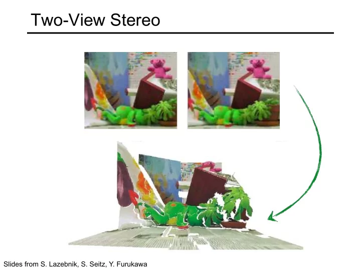
two view stereo
play

Two-View Stereo Slides from S. Lazebnik, S. Seitz, Y. Furukawa - PowerPoint PPT Presentation

Two-View Stereo Slides from S. Lazebnik, S. Seitz, Y. Furukawa Stereo What cues tell us about scene depth? Slide from L. Lazebnik. Stereograms Humans can fuse pairs of images to get a sensation of depth Stereograms: Invented by Sir


  1. Two-View Stereo Slides from S. Lazebnik, S. Seitz, Y. Furukawa

  2. Stereo • What cues tell us about scene depth? Slide from L. Lazebnik.

  3. Stereograms • Humans can fuse pairs of images to get a sensation of depth Stereograms: Invented by Sir Charles Wheatstone, 1838 Slide from L. Lazebnik.

  4. Stereograms Slide from L. Lazebnik.

  5. Stereograms • Humans can fuse pairs of images to get a sensation of depth Autostereograms: www.magiceye.com Slide from L. Lazebnik.

  6. Stereograms • Humans can fuse pairs of images to get a sensation of depth Autostereograms: www.magiceye.com Slide from L. Lazebnik.

  7. Problem formulation • Given a calibrated binocular stereo pair, fuse it to produce a depth image image 1 image 2 Dense depth map Slide from L. Lazebnik.

  8. Basic stereo matching algorithm • For each pixel in the first image • Find corresponding epipolar line in the right image • Examine all pixels on the epipolar line and pick the best match • Triangulate the matches to get depth information • Simplest case: epipolar lines are corresponding scanlines • When does this happen? Slide from L. Lazebnik.

  9. Simplest Case: Parallel images • Image planes of cameras are parallel to each other and to the baseline • Camera centers are at same height • Focal lengths are the same Slide from L. Lazebnik.

  10. Simplest Case: Parallel images • Image planes of cameras are parallel to each other and to the baseline • Camera centers are at same height • Focal lengths are the same • Then epipolar lines fall along the horizontal scan lines of the images Slide from L. Lazebnik.

  11. Essential matrix for parallel images Epipolar constraint: ¢ T = = x E x 0 , E [ t ] R ´ R = I t = ( T , 0, 0) x é ù 0 0 0 x’ ê ú = = - E [ t ] R 0 0 T ê ú ´ t ê ú 0 T 0 ë û é ù æ ö æ ö 0 0 0 u 0 ç ÷ ç ÷ ê ú ( ) ( ) ¢ ¢ ¢ ¢ ¢ - = - = = u v 1 0 0 T v 0 u v 1 T 0 T v Tv ç ÷ ç ÷ ê ú ç ÷ ç ÷ ê ú 0 T 0 1 Tv ë û è ø è ø The y-coordinates of corresponding points are the same!

  12. Stereo image rectification Slide from L. Lazebnik.

  13. Stereo image rectification • Reproject image planes onto a common plane parallel to the line between optical centers C. Loop and Z. Zhang. Computing Rectifying Homographies for Stereo Vision. CVPR 1999 Slide from L. Lazebnik.

  14. Rectification example Slide from L. Lazebnik.

  15. Another rectification example Unrectified Rectified Slide from L. Lazebnik.

  16. Basic stereo matching algorithm • If necessary, rectify the two stereo images to transform epipolar lines into scanlines • For each pixel in the first image • Find corresponding epipolar line in the right image • Examine all pixels on the epipolar line and pick the best match Slide from L. Lazebnik.

  17. Correspondence search Left Right scanline Matching cost disparity • Slide a window along the right scanline and compare contents of that window with the reference window in the left image • Matching cost: SSD or normalized correlation Slide from L. Lazebnik.

  18. Correspondence search Left Right scanline SSD Slide from L. Lazebnik.

  19. Correspondence search Left Right scanline Norm. corr Slide from L. Lazebnik.

  20. Basic stereo matching algorithm • If necessary, rectify the two stereo images to transform epipolar lines into scanlines • For each pixel x in the first image • Find corresponding epipolar scanline in the right image • Examine all pixels on the scanline and pick the best match x ’ • Triangulate the matches to get depth information Slide from L. Lazebnik.

  21. Depth from disparity X x f = B f = B 2 x − " 1 z z z x − " x = B 1 + B 2 x x’ f z f f B 1 B 2 × O Baseline O’ B f ¢ = - = disparity x x B z Disparity is inversely proportional to depth! Slide from L. Lazebnik.

  22. Depth from disparity X x f = B x f = B 2 ! 1 z z z x − " x = B 1 − B 2 x x’ f z f f B × O’ O B f ¢ = - = disparity x x z B 1 B 2 Slide from L. Lazebnik.

  23. Basic stereo matching algorithm • If necessary, rectify the two stereo images to transform epipolar lines into scanlines • For each pixel x in the first image • Find corresponding epipolar scanline in the right image • Examine all pixels on the scanline and pick the best match x ’ • Compute disparity x–x’ and set depth( x ) = B * f /( x–x’ ) Slide from L. Lazebnik.

  24. Failures of correspondence search Occlusions, repetition Textureless surfaces Non-Lambertian surfaces, specularities Slide from L. Lazebnik.

  25. Effect of window size W = 3 W = 20 • Smaller window + More detail – More noise • Larger window + Smoother disparity maps – Less detail Slide from L. Lazebnik.

  26. Results with window search Data Window-based matching Ground truth Slide from L. Lazebnik.

  27. Better methods exist... Graph cuts Ground truth Y. Boykov, O. Veksler, and R. Zabih, Fast Approximate Energy Minimization via Graph Cuts, PAMI 2001 For the latest and greatest: http://www.middlebury.edu/stereo/ Slide from L. Lazebnik.

  28. How can we improve window-based matching? • The similarity constraint is local (each reference window is matched independently) • Need to enforce non-local correspondence constraints Slide from L. Lazebnik.

  29. Non-local constraints • Uniqueness • For any point in one image, there should be at most one matching point in the other image Slide from L. Lazebnik.

  30. Non-local constraints • Uniqueness • For any point in one image, there should be at most one matching point in the other image • Ordering • Corresponding points should be in the same order in both views Slide from L. Lazebnik.

  31. Non-local constraints • Uniqueness • For any point in one image, there should be at most one matching point in the other image • Ordering • Corresponding points should be in the same order in both views Ordering constraint doesn’t hold Slide from L. Lazebnik.

  32. Non-local constraints • Uniqueness • For any point in one image, there should be at most one matching point in the other image • Ordering • Corresponding points should be in the same order in both views • Smoothness • We expect disparity values to change slowly (for the most part) Slide from L. Lazebnik.

  33. Scanline stereo • Try to coherently match pixels on the entire scanline • Different scanlines are still optimized independently Left image Right image Slide from L. Lazebnik.

  34. “Shortest paths” for scan-line stereo I ¢ Left image I Right image S left Right occlusion C q c occl o r r e occlusion s p Left o n d e t n c e C C corr S occl right s p Can be implemented with dynamic programming Ohta & Kanade ’85, Cox et al. ‘96 Slide credit: Y. Boykov Slide from L. Lazebnik.

  35. Coherent stereo on 2D grid • Scanline stereo generates streaking artifacts • Can’t use dynamic programming to find spatially coherent disparities/ correspondences on a 2D grid Slide from L. Lazebnik.

  36. Stereo matching as global optimization I 2 D I 1 W 1 ( i ) W 2 ( i+D ( i )) D ( i ) 2 + λ ( ) ( ) E ( D ) = W 1 ( i ) − W 2 ( i + D ( i )) ρ D ( i ) − D ( j ) ∑ ∑ i neighbors i , j data term smoothness term • Energy functions of this form can be minimized using graph cuts Y. Boykov, O. Veksler, and R. Zabih, Fast Approximate Energy Minimization via Graph Cuts, PAMI 2001 Slide from L. Lazebnik.

  37. Stereo matching as a prediction problem Y. Zhong, Y. Dai, and H. Li, Self-Supervised Learning for Stereo Matching with Self-Improving Ability, arXiv 2017 Slide from L. Lazebnik.

  38. Review: Basic stereo matching algorithm • For each pixel x in the reference image • Find corresponding epipolar scanline in the other image • Examine all pixels on the scanline and pick the best match x ’ • Compute disparity x–x’ and set depth( x ) = B * f /( x–x’ ) Slide from L. Lazebnik.

  39. Depth from Triangulation Camera 1 Camera 2 Camera Projector Passive Stereopsis Active Stereopsis Active sensing simplifies the problem of estimating point correspondences

  40. Kinect: Structured infrared light http://bbzippo.wordpress.com/2010/11/28/kinect-in-infrared/ Slide from L. Lazebnik.

  41. Apple TrueDepth https://www.cnet.com/new s/apple-face-id-truedepth- how-it-works/ Slide from L. Lazebnik.

  42. Laser scanning Digital Michelangelo Project Levoy et al. http://graphics.stanford.edu/projects/mich/ Optical triangulation • Project a single stripe of laser light • Scan it across the surface of the object • This is a very precise version of structured light scanning Source: S. Seitz

  43. Laser scanned models The Digital Michelangelo Project , Levoy et al. Source: S. Seitz

  44. Laser scanned models The Digital Michelangelo Project , Levoy et al. Source: S. Seitz

  45. Laser scanned models The Digital Michelangelo Project , Levoy et al. Source: S. Seitz

  46. Laser scanned models The Digital Michelangelo Project , Levoy et al. Source: S. Seitz

  47. Laser scanned models 1.0 mm resolution (56 million triangles) The Digital Michelangelo Project , Levoy et al. Source: S. Seitz

Download Presentation
Download Policy: The content available on the website is offered to you 'AS IS' for your personal information and use only. It cannot be commercialized, licensed, or distributed on other websites without prior consent from the author. To download a presentation, simply click this link. If you encounter any difficulties during the download process, it's possible that the publisher has removed the file from their server.

Recommend


More recommend