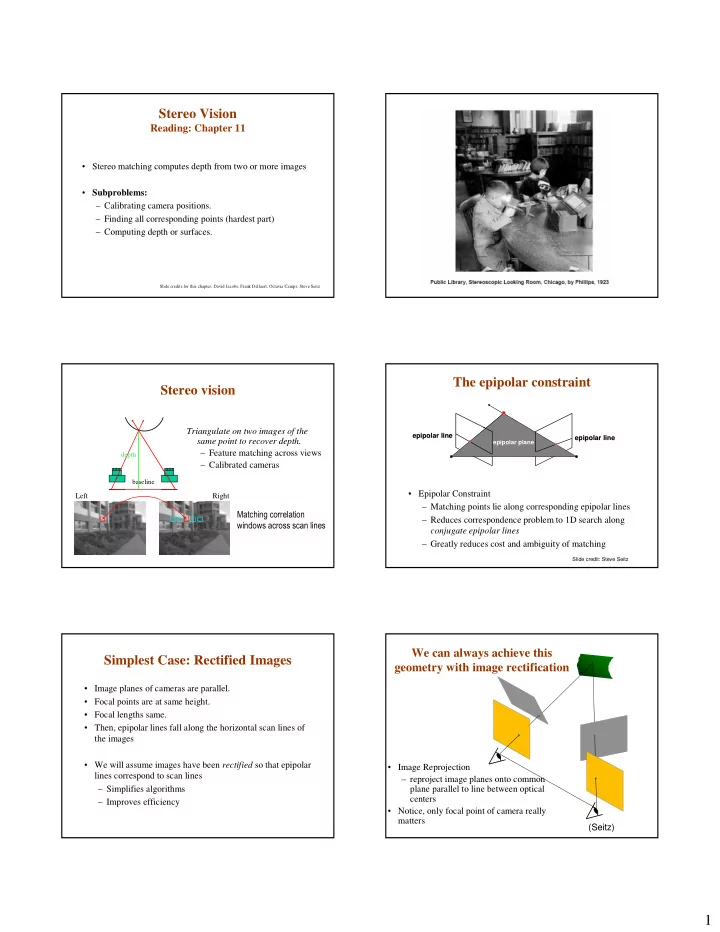
1 Basic Stereo Derivations Correspondence It is fundamentally - - PDF document

SLIDE 1

1

Stereo Vision

Reading: Chapter 11

• Stereo matching computes depth from two or more images
• Subproblems:

– Calibrating camera positions. – Finding all corresponding points (hardest part) – Computing depth or surfaces.

Slide credits for this chapter: David Jacobs, Frank Dellaert, Octavia Camps, Steve Seitz

Stereo vision

Triangulate on two images of the same point to recover depth. – Feature matching across views – Calibrated cameras

Left Right

baseline

• depth

The epipolar constraint

• Epipolar Constraint

– Matching points lie along corresponding epipolar lines – Reduces correspondence problem to 1D search along conjugate epipolar lines – Greatly reduces cost and ambiguity of matching

epipolar plane

epipolar line epipolar line epipolar line epipolar line

Slide credit: Steve Seitz

Simplest Case: Rectified Images

• Image planes of cameras are parallel.
• Focal points are at same height.
• Focal lengths same.
• Then, epipolar lines fall along the horizontal scan lines of

the images

• We will assume images have been rectified so that epipolar

lines correspond to scan lines – Simplifies algorithms – Improves efficiency

We can always achieve this geometry with image rectification

• Image Reprojection

– reproject image planes onto common plane parallel to line between optical centers

• Notice, only focal point of camera really

matters (Seitz)

SLIDE 2

2

Basic Stereo Derivations

PL = (X,Y,Z)

OL x y z

(uL,vL)

OR x y z

(uR,vR)

b a s e l i n e B Disparity:

Correspondence

• It is fundamentally ambiguous, even with stereo constraints
• Correspondence: What should we match?
• Objects?
• Edges?
• Pixels?
• Collections of pixels?

Julesz: showed that recognition is not needed for stereo.

Correspondence: Epipolar constraint.

The epipolar constraint helps, but much ambiguity remains.

Correspondence: Photometric constraint

• Same world point has same intensity in both images.

– True for Lambertian surfaces

• A Lambertian surface has a brightness that is

independent of viewing angle – Violations:

• Noise
• Specularity
• Non-Lambertian materials
• Pixels that contain multiple surfaces

SLIDE 3

3

Pixel matching

For each epipolar line For each pixel in the left image

• compare with every pixel on same epipolar line in right image
• pick pixel with minimum match cost

This leaves too much ambiguity, so:

Improvement: match windows

(Seitz)

Correspondence Using Correlation

SSD error disparity Left Right scanline

Sum of Squared (Pixel) Differences

Left Right

L

w

R

w

L

I

R

I

∑

∈

− − = + ≤ ≤ − + ≤ ≤ − =

) , ( ) , ( 2 2 2 2 2

)] , ( ) , ( [ ) , , ( : disparity

• f

function a as difference intensity the measures cost SSD The } , | , { ) , ( : function window the define We pixels.

• f

windows by ing correspond are and

y x W v u R L r m m m m m R L

m

v d u I v u I d y x C y v y x u x v u y x W m m w w

L

w

R

w ) , (

L L y

x ) , (

L L

y d x −

m m

Image Normalization

• Even when the cameras are identical models, there can be

differences in gain and sensitivity.

• For these reason and more, it is a good idea to normalize the

pixels in each window:

pixel Normalized ) , ( ) , ( ˆ magnitude Window )] , ( [ pixel Average ) , (

) , ( ) , ( ) , ( 2 ) , ( ) , ( ) , ( ) , ( 1 y x W y x W v u y x W y x W v u y x W

m m m m m

I I I y x I y x I v u I I v u I I − − = = =

∑ ∑

∈ ∈

Images as Vectors

Left Right

L

w

R

w

m m L

w

L

w

row 1 row 2 row 3

m m m

“Unwrap” image to form vector, using raster scan order

Each window is a vector in an m2 dimensional vector space. Normalization makes them unit length.

Image Metrics

L

w ) (d wR

2 ) , ( ) , ( 2 SSD

) ( )] , ( ˆ ) , ( ˆ [ ) ( d w w v d u I v u I d C

R L y x W v u R L

m

− = − − =

∑

∈

(Normalized) Sum of Squared Differences Normalized Correlation

θ cos ) ( ) , ( ˆ ) , ( ˆ ) (

) , ( ) , ( NC

= ⋅ = − =

∑

∈

d w w v d u I v u I d C

R L y x W v u R L

m

) ( max arg ) ( min arg

2 *

d w w d w w d

R L d R L d

⋅ = − =

SLIDE 4

4

Stereo Results

Images courtesy of Point Grey Research

Window size

W = 3 W = 20

• Effect of window size
• Some approaches have been developed to use an adaptive

window size (try multiple sizes and select best match) (Seitz)

Stereo testing and comparisons

Ground truth Scene

• D. Scharstein and R. Szeliski. "A Taxonomy and Evaluation of Dense Two-

Frame Stereo Correspondence Algorithms," International Journal of Computer Vision, 47 (2002), pp. 7-42.

Scharstein and Szeliski

Results with window correlation

Window-based matching (best window size) Ground truth (Seitz)

Results with better method

State of the art method: Graph cuts Ground truth (Seitz)

SLIDE 5

5

Stereo Correspondences

… …

Left scanline Right scanline

Stereo Correspondences

… …

Left scanline Right scanline

Match Match Match Occlusion Disocclusion

Search Over Correspondences

Three cases: – Sequential – add cost of match (small if intensities agree) – Occluded – add cost of no match (large cost) – Disoccluded – add cost of no match (large cost)

Left scanline Right scanline Occluded Pixels Disoccluded Pixels

Stereo Matching with Dynamic Programming

Dynamic programming yields the

• ptimal path through grid. This is

the best set of matches that satisfy the ordering constraint

Occluded Pixels Left scanline Dis-occluded Pixels Right scanline

Start End

Dynamic Programming

• Efficient algorithm for solving sequential decision (optimal path) problems.

1 2 3 1 2 3 1 2 3

1 = t 2 = t 3 = t 1 = i 2 = i 3 = i

1 2 3

T t =

…

How many paths through this trellis?

T

3

Dynamic Programming

1 2 3 1 2 3 1 2 3

1 − t

C

t

C

1 + t

C

12

Π

22

Π

32

Π Suppose cost can be decomposed into stages:

j i

ij

state to state from going

• f

Cost = Π 1 = i 2 = i 3 = i

States:

SLIDE 6

6

Dynamic Programming

1 2 3 1 2 3 1 2 3

1 − t

C

t

C

1 + t

C

12

Π

22

Π

32

Π Principle of Optimality for an n-stage assignment problem:

)) ( ( min ) (

1 i

C j C

t ij i t −

+ Π = 2 = j 1 = i 2 = i 3 = i

Dynamic Programming

1 2 3 1 2 3 1 2 3

1 − t

C

t

C

1 + t

C

2 ) 2 ( =

t

b

)) ( ( min arg ) ( )) ( ( min ) (

1 1

i C j b i C j C

t ij i t t ij i t − −

+ Π = + Π = 2 = j 1 = i 2 = i 3 = i

Stereo Matching with Dynamic Programming

Scan across grid computing optimal cost for each node given its upper-left neighbors. Backtrack from the terminal to get the optimal path.

Occluded Pixels Left scanline Dis-occluded Pixels Right scanline Terminal

Stereo Matching with Dynamic Programming

Scan across grid computing optimal cost for each node given its upper-left neighbors. Backtrack from the terminal to get the optimal path.

Occluded Pixels Left scanline Dis-occluded Pixels Right scanline Terminal

Stereo Matching with Dynamic Programming

Scan across grid computing optimal cost for each node given its upper-left neighbors. Backtrack from the terminal to get the optimal path.

Occluded Pixels Left scanline Dis-occluded Pixels Right scanline Terminal

Scharstein and Szeliski

SLIDE 7

7

Segmentation-based Stereo

Hai Tao and Harpreet W. Sawhney

Another Example Result using a good technique

Right Image Left Image Disparity

View Interpolation Computing Correspondence

• Another approach is to match edges rather than windows of pixels:
• Which method is better?

– Edges tend to fail in dense texture (outdoors) – Correlation tends to fail in smooth featureless areas

Summary of different stereo methods

• Constraints:

– Geometry, epipolar constraint. – Photometric: Brightness constancy, only partly true. – Ordering: only partly true. – Smoothness of objects: only partly true.

• Algorithms:

– What you compare: points, regions, features?

• How you optimize:

– Local greedy matches. – 1D search. – 2D search.