Dense Stereo Some Slides by Forsyth & Ponce, Jim Rehg, Sing - - PowerPoint PPT Presentation

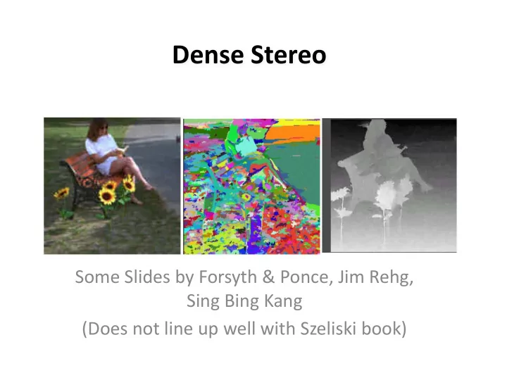
Dense Stereo

Some Slides by Forsyth & Ponce, Jim Rehg, Sing Bing Kang (Does not line up well with Szeliski book)

Etymology

Stereo comes from the Greek word for solid (stereo), and the term can be applied to any system using more than one channel

Effect of Moving Camera

• As camera is shifted

(viewpoint changed):

– 3D points are projected to different 2D locations – Amount of shift in projected 2D location depends

• n depth
• 2D shifts=Parallax

3D point

Basic Idea of Stereo

Triangulate on two images of the same point to recover depth.

– Feature matching across views – Calibrated cameras

Left Right

Matching correlation windows across scan lines

baseline depth

Why is Stereo Useful?

• Passive and non-

invasive

• Robot navigation

(path planning,

• bstacle detection)
• 3D modeling (shape

analysis, reverse engineering, visualization)

• Photorealistic

rendering

Outline

• Pinhole camera model
• Basic (2-view) stereo algorithm

– Equations – Window-based matching (SSD) – Dynamic programming

• Multiple view stereo

Review: Pinhole Camera Model

O Virtual image f x y z

P = (X,Y,Z) Q

3D scene point P is projected to a 2D point Q in the virtual image plane The 2D coordinates in the image are given by

(u,v)

Note: image center is (0,0)

(0,0)

Basic Stereo Derivations

PL = (X,Y,Z)

OL x y z

(uL,vL)

OR x y z

(uR,vR)

b a s e l i n e B Important note: Because the camera shifts along x, vL = vR

Basic Stereo Derivations

PL = (X,Y,Z)

OL x y z

(uL,vL)

OR x y z

(uR,vR)

b a s e l i n e B Disparity:

Stereo Vision

Left Right

Matching correlation windows across scan lines Z(x, y) is depth at pixel (x, y) d(x, y) is disparity

baseline depth

Z(x,y) = f B d(x,y)

Components of Stereo

• Matching criterion (error function)

– Quantify similarity of pixels – Most common: direct intensity difference

• Aggregation method

– How error function is accumulated – Options: Pixel, edge, window, or segmented regions

• Optimization and winner selection

– Examples: Winner-take-all, dynamic programming, graph cuts, belief propagation

Stereo Correspondence

• Search over disparity to find correspondences
• Range of disparities can be large

virtually no shift large shift

Correspondence Using Window-based Correlation

SSD error disparity Left Right scanline Matching criterion = Sum-of-squared differences Aggregation method = Fixed window size

“Winner-take-all”

Sum of Squared (Intensity) Differences

Left Right

wL and wR are corresponding m by m windows of pixels. We define the window function: Wm(x,y) = {u,v | x − m

2 ≤ u ≤ x + m 2 ,y − m 2 ≤ v ≤ y + m 2}

The SSD cost measures the intensity difference as a function of disparity: Cr(x,y,d) = [IL(u,v) − IR(u − d,v)]2

(u,v)∈Wm(x,y)

∑

Correspondence Using Correlation

Left Disparity Map Images courtesy of Point Grey Research

Image Normalization

• Images may be captured under different exposures (gain and

aperture)

• Cameras may have different radiometric characteristics
• Surfaces may not be Lambertian
• Hence, it is reasonable to normalize pixel intensity in each

window (to remove bias and scale):

I =

1 Wm(x,y)

I(u,v)

(u,v)∈Wm(x,y)

∑

Average pixel I Wm(x,y) = [I(u,v)]2

(u,v)∈Wm(x,y)

∑

Window magnitude ˆ I (x,y) = I(x,y) − I I − I

Wm(x,y)

Normalized pixel

Images as Vectors

Left Right row 1 row 2 row 3

“Unwrap” image to form vector, using raster scan order

Each window is a vector in an m2 dimensional vector space. Normalization makes them unit length.

Image Metrics

(Normalized) Sum of Squared Differences Normalized Correlation

q

CSSD(d) = [ˆ I

L(u,v) − ˆ

I

R(u − d,v)]2 (u,v)∈Wm(x,y)

∑

= wL − wR(d)

2

CNC(d) = ˆ I

L(u,v)ˆ

I

R(u − d,v) (u,v)∈Wm(x,y)

∑

= wL ⋅ wR(d) = cosθ

d* = argmind wL − wR(d)

2 = argmaxd wL ⋅ wR(d)

wR(d)

wL

Caveat

• Image normalization should be used only

when deemed necessary

• The equivalence classes of things that look

“similar” are substantially larger, leading to more matching ambiguities

x I x I x I x I Direct intensity Normalized intensity

Alternative: Histogram Warping

Cox, Roy, & Hingorani’95: “Dynamic Histogram Warping” (Assumes significant visual overlap between images) I freq I freq I freq I freq Compare and warp towards each other

Two major roadblocks

• Textureless regions create ambiguities
• Occlusions result in missing data

Textureless regions Occluded regions

Dealing with ambiguities and occlusion

• Ordering constraint:

– Impose same matching order along scanlines

• Uniqueness constraint:

– Each pixel in one image maps to unique pixel in

• ther
• Can encode these constraints easily in

dynamic programming

Pixel-based Stereo

… …

Left scanline Right scanline Center of left camera Center of right camera (NOTE: I’m using the actual, not virtual, image here.)

Stereo Correspondences

… …

Left scanline Right scanline

Match Match Match Occlusion Disocclusion

• Right image is reference
• Definition of
• cclusion/disocclusion

depends on which image is considered the reference

• Moving from left to right:

Pixels that “disappear” are occluded; pixels that “appear” are disoccluded

Search Over Correspondences

Three cases:

–Sequential – cost of match –Occluded – cost of no match –Disoccluded – cost of no match

Left scanline Right scanline Occluded Pixels Disoccluded Pixels

Stereo Matching with Dynamic Programming

Dynamic programming yields the optimal path through grid. This is the best set of matches that satisfy the ordering constraint

Occluded Pixels Left scanline Dis-occluded Pixels Right scanline

Start End

Ordering Constraint is not Generally Correct

• Preserves matching order along scanlines, but

cannot handle “double nail illusion”

A

• Slanted plane: Matching between M pixels

and N pixels

Uniqueness Constraint is not Generally Correct

Edge-based Stereo

• Another approach is to match edges rather than windows
• f pixels:
• Which method is better?

– Edges tend to fail in dense texture (outdoors) – Correlation tends to fail in smooth featureless areas – Sparse correspondences

Segmentation-based Stereo

Hai Tao and Harpreet W. Sawhney

Another Example

Hallmarks of A Good Stereo Technique

• Should not rely on order and uniqueness constraints
• Should account for occlusions
• Should account for depth discontinuity
• Should have reasonable shape priors to handle

textureless regions (e.g., planar or smooth surfaces)

• Should account for non-Lambertian surfaces
• There’s a database with ground truth for testing:

http://cat.middlebury.edu/stereo/data.html

Left Disparity Map Right

Result of using a more sophisticated stereo algorithm

View Interpolation

Result using a good technique

Right Image Left Image Disparity

View Interpolation

Bottom Line: Stereo is Still Unresolved

• Depth discontinuities
• Lack of texture (depth

ambiguity)

• Non-rigid effects

(highlights, reflection, translucency)

From 2 views to >2 views

• More pixels voting for the

right depth

• Statistically more robust
• However, occlusion

reasoning is more complicated, since we have to account for partial

• cclusion:

– Which subset of cameras sees the same 3D point?