SSA Static Single Assignment (SSA) was developed by R. Cytron, J. - - PDF document

4/3/2013 1

CS 2210: Static Single Assignment

Jonathan Misurda jmisurda@cs.pitt.edu

SSA

Static Single Assignment (SSA) was developed by R. Cytron, J. Ferrante, et al. in the 1980s. Every variable is statically assigned exactly one time in the source code (although that statement may execute many times at runtime).

• That is, there is only one def (definition) of a particular variable.

What about code like: x := 0 x := x + 1 Convert original variable name to nameversion (x → x1, x2) in different places as it is assigned to: x1 := 0 x2 := x1 + 1

Multiple Paths

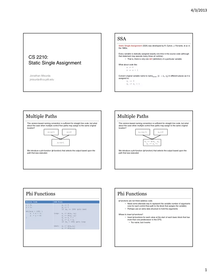
This version-based naming convention is sufficient for straight line code, but what about the case when multiple control flow paths may assign to the same original location? We introduce a phi-function (ϕ-function) that selects the output based upon the path that was executed. x:=x+1 x:=0 x:=x+1

Multiple Paths

This version-based naming convention is sufficient for straight line code, but what about the case when multiple control flow paths may assign to the same original location? We introduce a phi-function (ϕ-function) that selects the output based upon the path that was executed. x2:=x1+1 x3:=0 x4 := ϕ(x2, x3) x5 := x4 +1

Phi Functions

Source Code SSA Form x = 0; y = 1; while(x < 100) { x = x + 1; y = y + x; } x0 := 0 y0 := 1 if (x0 >= 100) goto next loop: x1 := ϕ(x0, x2) y1 := ϕ(y0, y2) x2 := x1 + 1 y2 := y1 + x2 if (x2 < 100) goto loop next: x3 := ϕ(x0,x2) y3 := ϕ(y0,y2)

Phi Functions

ϕ-functions are not three-address code.

• Need some alternate way to represent the variable number of arguments

(one for each control-flow path to the block that assigns the variable).

• Perhaps use an extra data structure to hold the arguments

Where to insert ϕ-functions?

• Insert ϕ-functions for each value at the start of each basic block that has

more than one predecessor in the CFG.

• Too naïve, but it works

4/3/2013 2

Path-Convergence Criterion

There should be a ϕ-function for variable a at node z of the flow graph exactly when all of the following are true:

• 1. There is a block x containing a definition of a,
• 2. There is a block y (with y ≠ x) containing a definition of a,
• 3. There is a nonempty path Pxz of edges from x to z,
• 4. There is a nonempty path Pyz of edges from y to z,
• 5. Paths Pxz and Pyz do not have any node in common other than z, and
• 6. The node z does not appear within both Pxz and Pyz prior to the end, though it

may appear in one or the other.

Iterated Path-Convergence

The start node contains an implicit definition of every variable

• formal parameters
• a ←uninitialized

A ϕ-function also counts as a definition of a, so the path-convergence criterion must be considered as a set of equations to be solved by iteration. while there are nodes x, y, z satisfying conditions 1–5 and z does not contain a ϕ-function for a do insert a ← ϕ(a, a, . . ., a) at node Z where the ϕ-function has as many a arguments as there are predecessors of node z.

Iterated Path-Convergence

The iterated path-convergence algorithm for placing ϕ-functions is not practical

• Must examine every triple of nodes x, y, z and
• Every path leading from x and y.

A much more efficient algorithm uses the dominator tree of the control flow graph.

Dominators

Certain blocks dominate other blocks in control flow graphs

• All paths from the root to a given basic block must go through the

dominator Example: Block 1 dominates blocks 2 and 3 If a block A dominates another block B, then we do not need a ϕ-function as we know one of two things:

• The definitions of variables in A reach into B, unless
• A redefinition of a variable happens in the path between A and B

1 2 3

Basic Dominator Algorithm

Dominators[r] = {r} foreach node n ∈ (N - r) Dominators[n] = N do changed = false foreach node n ∈ (N - r) T = N foreach node p in Predecessors(n) { T = T ∩ Dominators[p] D = T ∪ n if ( D != Dominators[n] ) changed = true Dominators[n] = D until(!changed)

Input: N = set of nodes in CFG r = root of CFG Output: Set of Dominator sets for each CFG node

Sample CFG

long evenSum=0; int i=0; while(i<1000000) { if(i%2 == 0){ evenSum+=i; } i++; } return;

evenSum+=i; if(i%2 == 0) i++; while(i<1000000) return; long evenSum=0; int i=0;

4/3/2013 3

Dominators

evenSum+=i; if(i%2 == 0) i++; while(i<1000000) return; long evenSum=0; int i=0;

1 2 3 4 5 6

The root dominates itself. Dom(1) = {1} Dom(2) = {1, 2} Dom(3) = {1, 2, 3} Dom(4) = {1, 2, 3, 4} Not all paths to 5 go through 4, so: Dom(5) = {1, 2, 3, 5} Dom(6) = {1, 2, 6}

Strict & Immediate Dominance

a strictly dominates b if

• 1. a dom b and
• 2. a ≠ b.

For a ≠ b, a immediately dominates b if and only if:

• 1. a dom b, and
• 2. there does not exist a node c such that:
• a. c ≠ a and c ≠ b
• b. a dom c and c dom b.

Thus, a idom b means that the closest dominator of b to the root (travelling backwards from b along the reverse control flow edges) is a. The immediate dominator of a node is unique.

Immediate Dominator Algorithm

temp = {} foreach node n ∈ N temp[n] = Dominators[n] - {n} foreach node n ∈ (N - {r}) foreach node s ∈ temp[n] foreach node t ∈ (temp[n] - {s}) if(t ∈ temp[s]) { temp[n] -= {t} foreach node n ∈ (N - {r}) idom[n] = temp[n]

Input: N = set of nodes in CFG Dominators[x] = Dominators

• f x

r = root of CFG Output: Immediate dominator for each CFG node

Dominators

evenSum+=i; if(i%2 == 0) i++; while(i<1000000) return; long evenSum=0; int i=0;

1 2 3 4 5 6

Dom(1) = {1} Dom(2) = {1, 2} Dom(3) = {1, 2, 3} Dom(4) = {1, 2, 3, 4} Dom(5) = {1, 2, 3, 5} Dom(6) = {1, 2, 6} idom(1) = {} idom(2) = {1} idom(3) = {2} idom(4) = {3} idom(5) = {3} idom(6) = {2}

Dominator Tree

The immediate dominance relation forms a tree of the nodes of a flowgraph where:

• 1. The root is the entry node,
• 2. The edges are immediate dominances, and
• 3. The paths display all of the dominance relationships.

evenSum+=i; if(i%2 == 0) i++; while(i<1000000) return; long evenSum=0; int i=0;

1 2 3 4 5 6

idom(1) = {} idom(2) = {1} idom(3) = {2} idom(4) = {3} idom(5) = {3} idom(6) = {2}

1 2 3 6 4 5

Dominance Frontier

The dominance frontier of a node a is the set of all nodes s such that a dominates a predecessor of s, but does not strictly dominate s. It is the “border” between dominated and undominated nodes. 1 2 3 4 13 5 6 7 8 9 10 11 12 Node 5 dominates the shaded nodes. The dominance frontier is those nodes who are not strictly dominated by 5. DF[5] = {4, 5, 12, 13}

4/3/2013 4

Dominance Frontier

A definition in node n forces a φ-function at join points that lie just outside the region of the CFG that n dominates. A definition in node n forces a corresponding φ-function at any join point m where:

• 1. n dominates a predecessor of m (q ∈ preds(m) and n ∈ Dom(q)), and
• 2. n does not strictly dominate m.

(Using strict dominance rather than dominance allows a φ-function at the start of a single-block loop. In that case, n=m, and m ∉ Dom(n) – {n}.) We call the collection of nodes m that have this property with respect to n the dominance frontier of n, denoted DF(n).

Dominance Frontier Criterion

Whenever node x contains a definition of some variable a, then any node z in the dominance frontier of x needs a φ-function for a. Since a φ-function itself is a definition, we must iterate the dominance-frontier criterion until there are no nodes that need φ-functions. The iterated dominance frontier criterion and the iterated path convergence criterion specify exactly the same set of nodes at which to put φ-functions.

Computing the Dominance Frontier

Alternative Algorithm:

foreach node n in the CFG DF(n) = {} foreach node n in the CFG if(n has multiple predecessors) foreach predecessor p of n runner = p while(runner ≠ IDom(n)) DF(runner) = DF(runner) ∪ {n} runner = IDom(runner)

Dominance Frontier

evenSum+=i; if(i%2 == 0) i++; while(i<1000000) return; long evenSum=0; int i=0;

1 2 3 4 5 6

1 2 3 6 4 5 Block n=1: Has No Predecessors DF(1) = {} Block n=2: Has multiple predecessors (1,5) Runner = 1 IDom(2) = 1 # Done with 1 Runner = 5 IDom(2) = 1 DF(5) = {} + {2} = {2} Runner = IDom(Runner) = 3 DF(3) = {} + {2} = {2} Runner = IDom(Runner) = 2 DF(2) = {} + {2} = {2} Runner = IDom(Runner) = 1 # Done

Dominance Frontier

evenSum+=i; if(i%2 == 0) i++; while(i<1000000) return; long evenSum=0; int i=0;

1 2 3 4 5 6

1 2 3 6 4 5 Block n=3: Has 1 predecessor DF(3) = {2} Block n=4: Has 1 predecessor DF(4) = {} Block n=5: Has 2 predecessors (3,4) Runner = 3 IDom(5) = 3 # Done with 3 Runner = 4 IDom(5) = 3 DF(4) = {} + {5} Runner = IDom(Runner) = 3 IDom(5) = 3 # Done with 4 Block n=6: Has 1 predecessor DF(6) = {}

DF(1)={} DF(2)={2} DF(3)={2} DF(4)={5} DF(5)={2} DF(6)={}

Inserting φ-Functions

Starting with a program not in SSA form, we need to insert just enough φ-functions to satisfy the iterated dominance frontier criterion. Start with a set V of variables, a graph G of control-flow nodes, and for each node n a set Aorig[n] of variables defined in node n. Compute Aφ[a], the set of nodes that must have φ-functions for variable a. Use a work list W of nodes that might violate the dominance-frontier criterion.

4/3/2013 5

Placing Phi Functions

Place-φ-Functions = foreach node n foreach variable a in Aorig[n] defsites[a] ← defsites[a] ∪ {n} foreach variable a W ← defsites[a] while W not empty remove some node n from W foreach y in DF[n] if(a ∉ Aφ[y]) insert the statement a ←φ(a, a, … , a) at the top of block y, where the φ-function has as many arguments as y has predecessors Aφ[Y] ← Aφ[Y] ∪ {a} if(a ∈ Aorig[y]) W ← W ∪ {y}

Inserting φ-Functions

evenSum+=i; if(i%2 == 0) i++; while(i<1000000) return; long evenSum=0; int i=0;

1 2 3 4 5 6

1 2 3 6 4 5 V = {evenSum, i} Def[evenSum] = {1, 4} Def[i] = {1, 5} For evenSum: W = {1, 4} n = 1 DF[1] = {} #Done n = 4 DF[4] = {5} Insert φ into block 5 for evenSum For i: W = {1,5} n = 1 DF[1] = {} #Done n = 5 DF[5] = {2} Insert φ into block 2 for i

DF(1)={} DF(2)={2} DF(3)={2} DF(4)={5} DF(5)={2} DF(6)={}

CFG with φ-Functions

evenSum+=i; if(i%2 == 0) evenSum = φ(evenSum, evenSum) i++; i = φ(i, i) while(i<1000000) return; long evenSum=0; int i=0;

1 2 3 4 5 6

Renaming the Variables

After the φ-functions are placed, we can walk the dominator tree, renaming the different definitions (including φ-functions) of variable a to a1, a2, a3, and so on. In a straight-line program, we would rename all the definitions of a, and then each use of a is renamed to use the most recent definition of a. For a program with control-flow branches and joins whose graph satisfies the dominance-frontier criterion, we rename each use of a to use the closest definition d of a that is above a in the dominator tree.

Renaming Variables (I)

Initialization: foreach variable a Count[a] ← 0 Stack[a] ← empty push 0 onto Stack[a] Rename(n) = foreach statement S in block n if S is not a φ-function foreach use of some variable x in S i ← top(Stack[x]) replace the use of x with xi in S foreach definition of some variable a in S Count[a] ← Count[a] + 1 i ← Count[a] push i onto Stack[a] replace definition of a with definition of ai in S

Renaming Variables (II)

foreach successor Y of block n, Suppose n is the jth predecessor of Y foreach φ-function in Y suppose the jth

• perand of the φ-function is a

i ←top(Stack[a]) replace the jth

• perand with ai

foreach child X of n in the dominator tree Rename(X) foreach statement S in block n foreach definition of some variable a in S pop Stack[a]

4/3/2013 6

Numbering

evenSum+=i; if(i%2 == 0) evenSum = φ(evenSum, evenSum) i++; i = φ(i, i) while(i<1000000) return; evenSum=0; i1=0;

Just done for variable i in this example Count[i] = 0 Stack[i] = 0 Rename(1) For each statement, if it’s not a φ-function, for each use of variable x, use the top of the stack’s number For each definition of a variable Count[i] = Count[i] + 1 = 1 Stack[i] = [1,0] 1 2 3 4 5 6

Numbering

evenSum+=i; if(i%2 == 0) evenSum = φ(evenSum, evenSum) i++; i = φ(i1, i) while(i<1000000) return; evenSum1=0; i1=0;

Count[i] = Count[i] + 1 = 1 Stack[i] = [1,0] Rename(1) For each successor of block 1: {2} For each φ-function Replace the corresponding parameter of the φ-function with the current subscripted version Recurse on each child in the IDom tree 1 2 3 4 5 6

Numbering

evenSum+=i2; if(i2%2 == 0) evenSum = φ(evenSum, evenSum) i=i2+1; i2 = φ(i1, i) while(i2<1000000) return; evenSum1=0; i1=0;

Rename(2) Skip φ-function Count[i] = Count[i] + 1 = 2 Stack[i] = [2,1,0] Subscript the definition with top of stack Subscript use in second statement Rename(3) Subscript use in statement Rename(4) Subscript use in statement Rename(4) Subscript use in statement 1 2 3 4 5 6

Numbering

evenSum+=i2; if(i2%2 == 0) evenSum = φ(evenSum, evenSum) i3=i2+1; i2 = φ(i1, i3) while(i2<1000000) return; evenSum1=0; i1=0;

Rename(5) Skip φ-function Subscript use in second statement Subscript def with new count Push new subscript into the successor’s φ- function 1 2 3 4 5 6

Speed of SSA Conversion

The DF computation does work proportional to the size (number of edges) of the

• riginal graph, plus the size of the dominance frontiers it computes. In practice, this

is usually linear in the size of the graph. The placing of phi functions algorithm does a constant amount of work for

• 1. each node and edge in the CFG,
• 2. each statement in the program,
• 3. each element of every dominance frontier, and
• 4. each inserted φ-function.

For a program of size N:

• the amounts (1) and (2) are proportional to N,
• (3) is usually approximately linear in N
• (4) could be N2 in the worst case, but empirical measurement has shown

that it is usually proportional to N.

Speed of SSA Conversion

Renaming takes time proportional to the size of the program (after φ-functions are inserted), so in practice it should be approximately linear in the size of the original program. The algorithms for computing SSA from the dominator tree are thus quite efficient. But the iterative set-based algorithm for computing dominators, may be slow in the worst case The Lengauer-Tarjan algorithm is a nearly linear-time algorithm that computes the dominator tree based upon the depth-first search spanning tree of the CFG.

4/3/2013 7

Converting out of SSA

After program transformations and optimization, a program in SSA form must be translated into some executable representation without φ-functions. The definition y ←φ(x1, x2, x3) can be translated as:

• move y ← x1 if arriving along predecessor edge 1,
• move y ← x2 if arriving along predecessor edge 2, and
• move y ← x3 if arriving along predecessor edge 3.

It is tempting simply to assign x1 and x2 the same register if they were derived from the same variable x. However, transformations on SSA form may make live ranges interfere. Instead, we rely on coalescing in the register allocator to eliminate almost all of the move instructions.