SSA form Static single assignment (SSA) form Michel Schinz - - PDF document

▶

Jan 29, 2023 153 likes •244 views

SSA form Static single assignment (SSA) form Michel Schinz Advanced Compiler Construction 2008-05-23 Static single assignment Straight-line code Transforming a piece of straight-line code i.e. without branches to SSA is trivial:

SLIDE 1

SSA form

Michel Schinz Advanced Compiler Construction – 2008-05-23

Static single assignment (SSA) form

Static single assignment

Static single-assignment (or SSA) form is an intermediate representation in which each variable has only one definition in the program. That single definition can be executed many times when the program is run – if it is inside a loop – hence the qualifier static. SSA form is interesting because it simplifies several

ptimisations and analysis, as we will see.

Straight-line code

Transforming a piece of straight-line code – i.e. without branches – to SSA is trivial: each definition of a given name gives rise to a new version of that name, identified by a subscript:

x=12 y=15 x=x+y y=x+4 z=x+y y=y+1 x1=12 y1=15 x2=x1+y1 y2=x2+4 z1=x2+y2 y3=y2+1 to SSA

functions

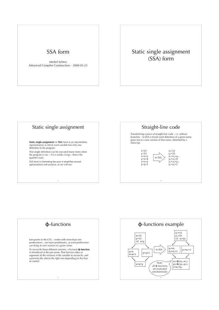
Join-points in the CFG – nodes with more than one predecessors – are more problematic, as each predecessor can bring its own version of a given name. To reconcile those different versions, a fictional -function is introduced at the join point. That function takes as argument all the versions of the variable to reconcile, and automatically selects the right one depending on the flow

f control.

functions example

x=12 y=15 if x<y y=x x=x+1 y=x+1 z=x*y x1=12 y1=15 if x1<y1 y2=x1 x2=x1+1 y3=x1+1 x3=(x2,x1) y4=(y2,y3) z=x3*y4 to SSA Note: all functions are evaluated simultaneously

SLIDE 2

(Naïve) building of SSA form

Naïve technique to build SSA form:

for each variable x of the CFG, at each join point n,

insert a -function of the form x=(x,…,x) with as many parameters as n has predecessors,

compute reaching definitions, and use that information

to rename any use of a variable according to the – now unique – definition reaching it.

(Naïve) building of SSA form

CFG

x=1 y=2 z=x+y y=y-1 x=x+y y=y+1 x=y y=x*2 z=z+x

After phase 1

x=1 y=2 z=x+y y=y-1 x=x+y y=y+1 x=y x=(x,x) y=(y,y) z=(z,z) y=x*2 z=z+x

After phase 2

x1=1 y1=2 z1=x1+y1 y2=y1-1 x2=x1+y2 y3=y1+1 x3=y3 x4=(x2,x3) y4=(y2,y3) z2=(z1,z1) y5=x4*2 z3=z2+x4

dead redundant

Smarter techniques

The naïve technique just presented works, in the sense that the resulting program is in SSA form and is equivalent to the original one. However, it introduces too many -functions – some dead, some redundant – to be useful in practice. It builds the maximal SSA form. We will examine better techniques later, but to understand them we must first introduce the notion of dominance in a CFG.

Dominance

In a control-flow graph, a node n1 dominates a node n2 if all paths from the start node to n2 pass through n1. By definition, the domination relation is reflexive, that is a node n always dominates itself. We then say that node n1 strictly dominates n2 if n1 dominates n2 and n1 n2. The immediate dominator of a node n is the strict dominator of n closest to n.

Dominance example

CFG 1 2 3 4 5 6 7 Dominance Node Dominators { 0 } 1 { 0, 1 } 2 { 0, 1, 2 } 3 { 0, 1, 3 } 4 { 0, 1, 3, 4 } 5 { 0, 1, 3, 5 } 6 { 0, 1, 3, 6 } 7 { 0, 1, 7 } (immediate dominator in bold)

SLIDE 3

Dominator tree

The dominator tree is a tree representing the dominance relation. The nodes of the tree are the nodes of the CFG, and a node n1 is a parent of a node n2 if and only if n1 is the immediate dominator of n2.

Dominator tree example

CFG 1 2 3 4 5 6 7 Dominator tree 1 2 3 4 5 6 7

Computing dominance

Dominance can be computed using data-flow analysis. To each node n of the CFG we attach a variable vn giving the set of nodes that dominate n. The value of vn is given by the following equation: vn = { n } (vp1 vp2 … vpk) where p1, …, pk are the predecessors of n.

Dominance frontier

The dominance frontier of a node n – written DF(n) – is the set of all nodes m such that n dominates a predecessor of m, but does not strictly dominates m itself. Informally, the dominance frontier of n contains the first nodes which are reachable from n but which are not strictly dominated by n.

Dominance frontier example

Dominance frontier CFG 1 2 3 4 5 6 7 7 6 5 4 3 2 1 dominance frontier of 3={7} nodes dominated by 3

Building SSA form

SLIDE 4

Minimal SSA form

The naïve technique to build SSA form presented earlier inserts -functions for every variable at the beginning of every join point. Using dominance information, it is possible to do better, and compute minimal SSA form: for each definition of a variable x in a node n, insert a -function for x in all nodes

f DF(n).

Notice that the inserted -functions are definitions, and can therefore force the insertion of more -functions.

Improving on minimal SSA

Reminder: the naïve technique to build SSA form presented at the beginning computes maximal SSA form. The better technique just presented computes minimal SSA form. Unfortunately, minimal SSA form is not necessarily optimal, and can contain dead -functions. To solve that problem, improved techniques have been developed to build semi- pruned – which is still not optimal – and pruned SSA form.

Semi-pruned SSA form

Observation: a variable that is only live in a single node can never have a live -function. Therefore, the minimal technique can be further refined by first computing the set of global names – defined as the names that are live across more than one node – and producing -functions for these names only. This is called semi-pruned SSA form.

Building semi-pruned SSA form

Like the naïve technique to build maximal SSA form, the algorithm to build semi-pruned SSA form is composed of two phases:

1. -functions are inserted for global names, according

to dominance information,

2. variables are renamed.

Phase 1: inserting -functions

Before inserting -functions, the set G of global names must be computed. Once this is done, insertion of - functions is done as follows: for each name x in G work list = all nodes in which x is defined for each node n in work list for each node m in DF(n) insert a -function for x in m work list = work list { m }

Phase 2: renaming variables

Renaming is done by a pre-order traversal of the dominator tree, as follows: for each node n in the dominator tree rename definitions and uses of variables in n rename -functions parameters corresponding to n in all successors of n in the CFG.

SLIDE 5

CFG

Example: phase 1

Algorithm (phase 1)

for each name x in {x,y,z} work list = all nodes in which x is defined for each node n in work list for each node m in DF(n) insert a -function for x in m work list = work list { m }

b c

Result

wrk lst

fun.

[a,b,c] [b,c] for x in d [c,d] for x in d [d] [] name x wrk lst

fun.

[a,b,c,d] [b,c,d] for y in d [c,d] for y in d [d] [] name y wrk lst -fun. [a,d] [d] [] name z

x=1 y=2 z=x+y y=y-1 x=x+y y=y+1 x=y y=x*2 z=z+x a d DF(a) = DF(d) = {} DF(b) = DF(c) = {d} x=(x,x) y=(y,y)

CFG

Example: phase 2

Dominator tree

a b c d

Algorithm (phase 2)

for each node n in the dominator tree (pre-order) rename definitions and uses of variables in n rename -functions parameters corresponding to n in all successors of n in the CFG.

b c x=1 y=2 z=x+y x1=1 y1=2 z1=x1+y1 y=y-1 x=x+y y=y+1 x=y x=(x,x) y=(y,y) y=x*2 z=z+x a d chosen pre-order: a,b,d,c y2=y1-1 x2=x1+y2 y5=y1+1 x4=y1 x=(x2,x) y=(y2,y) y=x*2 z=z+x x3=(x2,x) y3=(y2,y) y4=x3*2 z2=z1+x3 x3=(x2,x4) y3=(y2,y5) y4=x3*2 z2=z1+x3

Generating code from SSA form

Generating code from SSA

After the program has been turned into SSA form and the various optimisations performed on that representation, it must be transformed into executable form. This implies in particular that -functions must be removed, as they cannot be implemented on standard machines.

Removing -functions

A -function of the form xi=(x1,…,xn) can be removed by inserting appropriate assignments to xi in all predecessors of the node containing that function. This will introduce many assignments of the form xi=xj (that is, move instructions), but most of them will be removed later during register allocation, thanks to coalescing.

Removing -functions

x1=12 y1=15 if x1<a1 y2=x1 x2=x1+1 y3=x1+1 x3=(x2,x1) y4=(y2,y3) z=x3*y4 x1=12 y1=15 if x1<a1 y2=x1 x2=x1+1 x3=x2 y4=y2 y3=x1+1 x3=x1 y4=y3 z=x3*y4

function

removal

SLIDE 6

Critical edges

CFG edges that go from a node with multiple successors to a node with multiple predecessors are called critical edges. While removing -functions, the presence of a critical edge from n1 to n2 leads to the insertion of redundant move instructions in n1, corresponding to the -functions of n2. Ideally, they should be executed only if control reaches n2 later, but this is not certain when n1 executes.

Edge splitting

Critical edges can easily be avoided completely using edge splitting. Edge splitting consists in replacing all critical edges leading from a node n1 to a node n2 by two edges: one from n1 to a new empty node n3, and one from n3 to n2. Since the new empty block n3 has only one predecessor and one successor, this effectively removes the critical edge.

Without edge splitting

x1=12 y1=15 if x1<y1 y2=x1 x2=x1+1 x3=(x2,x1) y3=(y2,y1) z=x3*y3

function

removal x1=12 y1=15 x3=x1 y3=y1 if x1<y1 y2=x1 x2=x1+1 x3=x2 y3=y2 z=x3*y3 potentially redundant critical edge

With edge splitting

x1=12 y1=15 if x1<y1 y2=x1 x2=x1+1 x3=(x2,x1) y3=(y2,y1) z=x3*y3

function

removal x1=12 y1=15 if x1<y1 y2=x1 x2=x1+1 x3=x2 y3=y2 x3=x1 y3=y1 z=x3*y3

Using SSA form

Dead-code elimination

Basic dead-code elimination is trivial in SSA form: if a variable xi is not used in some expression, then its definition –of the form xi=yj op zk or xi=(xj, …, xk) – can be deleted. Of course, this is only true if that definition does not have side-effects. The deletion of a definition can remove the last use of some

ther variable, in which case its definition can be deleted

too, and so on…

SLIDE 7

Simple constant propagation

SSA form also simplifies constant propagation: whenever a definition of the form xi=c – where c is a constant – is encountered, then all uses of xi can be replaced by c. Moreover, the definition itself can be deleted from the program, as it is now dead. Also, a -function of the form xi=(c1,…,cn) where c1=…=cn can be replaced by xi=c1, which is then simplified as above.

Copy propagation

Copy propagation can be handled in a similar fashion as constant propagation: definitions of the form xi=yj, and single-argument -functions of the form xi=(yj) can be deleted, and all uses of xi replaced by uses of yj. The same is true of constant folding: a definition of the form xi=c1 op c2 – where c1 and c2 are constants – can be deleted and all uses of xi replaced by the value of c1 op c2.

Liveness analysis

SSA form also simplifies liveness analysis, and hence the construction of the interference graph needed by register allocation. To compute the region where a variable xi is live in SSA form, it is sufficient to start from all uses of xi and walk backwards in the CFG until the definition of xi is

encountered. The statements encountered during that walk

are those during which xi is live.

Summary

Static single-assignment (SSA) form is an intermediate representation where all names are defined exactly once. To enable this, -functions have to be inserted at join points in the CFG. Transforming a program to SSA form is not completely trivial since unnecessary -functions should be avoided. SSA encodes the data-flow of the program in its names, making several optimisations easier.