Static Single Assignment Form Last Time Static single assignment - - PDF document

CS553 Lecture Static Single Assignment Form 1

Static Single Assignment Form

Last Time

– Static single assignment (SSA) form

Today

– Applications of SSA

CS553 Lecture Static Single Assignment Form 2

Dead Code Elimination for SSA

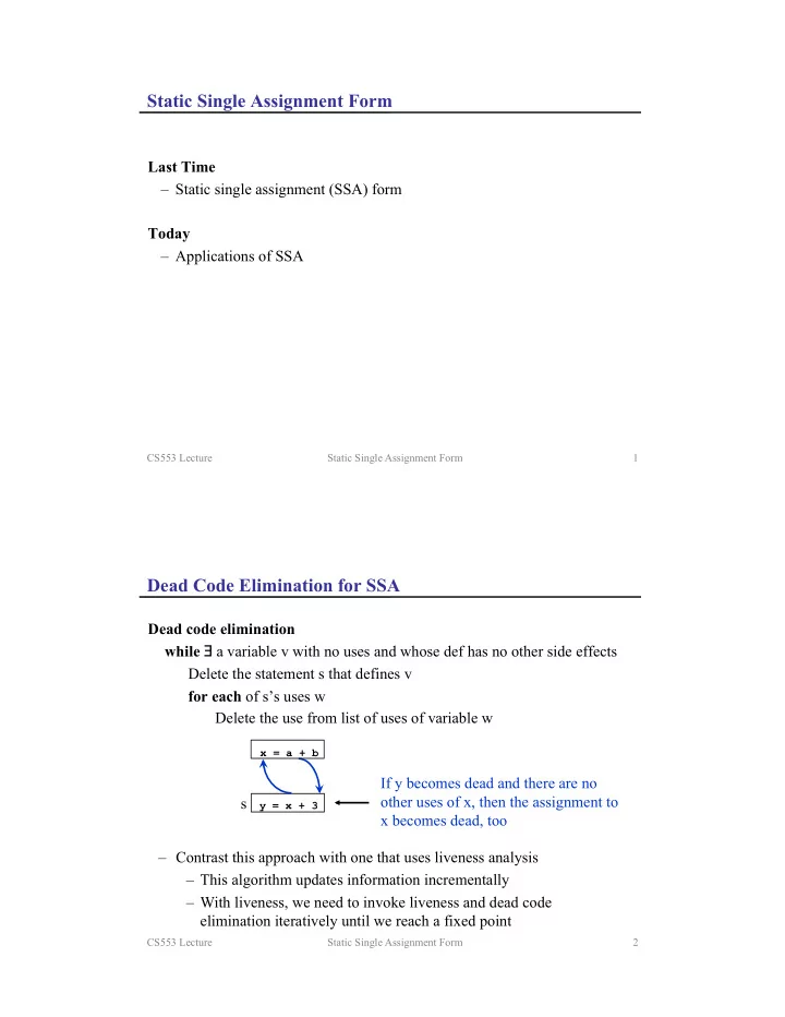
Dead code elimination

while a variable v with no uses and whose def has no other side effects Delete the statement s that defines v for each of s’s uses w Delete the use from list of uses of variable w

x = a + b

If y becomes dead and there are no

• ther uses of x, then the assignment to

x becomes dead, too – Contrast this approach with one that uses liveness analysis – This algorithm updates information incrementally – With liveness, we need to invoke liveness and dead code elimination iteratively until we reach a fixed point

y = x + 3

s

CS553 Lecture Static Single Assignment Form 3

Implementing Simple Constant Propagation

Standard worklist algorithm

– Identifies simple constants – For each program point, maintains one constant value for each variable Solution !Exploit a sparse dependence representation (e.g., SSA) Problem !Inefficient, since constants may have to be propagated through irrelevant nodes

x = 1 y = x

CS553 Lecture Static Single Assignment Form 4

Sparse Simple Constant Propagation

Reif and Lewis algorithm

– Identifies simple constants – Faster than Simple Constants algorithm SSA edges !Explicitly connect defs with uses !How would you do this? Main Idea !Iterate over SSA edges instead of

• ver all CFG edges

x = 1 y = x

CS553 Lecture Static Single Assignment Form 5

worklist = all statements in SSA while worklist Remove some statement S from worklist if S is x = phi(c,c,...,c) for some constant c replace S with v = c if S is x=c for some constant c delete S from program for each statement T that uses x substitute c for x in T worklist = worklist union {T}

Sparse Simple Constants Algorithm (Ch. 19 in Appel)

CS553 Lecture Static Single Assignment Form 6

Copy Propagation

Algorithm

worklist = all statements in SSA while worklist Remove some statement S from worklist if S is x = phi(y) or x = y for each statement T that uses x replace all use of x with y worklist = worklist union {T} delete S

CS553 Lecture Value Numbering 7

Reuse Optimization

Idea

– Eliminate redundant operations in the dynamic execution of instructions

How do redundancies arise?

– Loop invariant code (e.g., index calculation for arrays) – Sequence of similar operations (e.g., method lookup) – Same value be generated in multiple places in the code

Types of reuse optimization

– Value numbering – Common subexpression elimination – Partial redundancy elimination

CS553 Lecture Value Numbering 8

Local Value Numbering

Idea

– Each variable, expression, and constant is assigned a unique number – When we encounter a variable, expression or constant, see if it’s already been assigned a number – If so, use the value for that number – If not, assign a new number – Same number same value

Example a := b + c d := b b := a e := d + c b #1 c #2 b + c is #1 + # 2 #3 a #3 d #1 d + c is #1 + # 2 #3 e #3 #3 a

CS553 Lecture Value Numbering 9

Local Value Numbering (cont)

Temporaries may be necessary

a := b + c

• a := b
• d := a + c

b #1 c #2 b + c is #1 + # 2 #3 a #3 a + c is #1 + # 2 #3 d #3

t := b + c

• a := b
• d := b + c

b #1 c #2 b + c is #1 + # 2 #3 t #3 a #1 a + c is #1 + # 2 #3 d #3 #1 t

CS553 Lecture Value Numbering 10

Global Value Numbering

How do we handle control flow?

w = 8 x = 8 w = 5 x = 5 y = w+1 z = x+1 w #2 x #2 . . . w #1 x #1 . . .

CS553 Lecture Value Numbering 11

Global Value Numbering (cont)

Idea [Alpern, Wegman, and Zadeck 1988]

– Partition program variables into congruence classes – All variables in a particular congruence class have the same value – SSA form is helpful

Approaches to computing congruence classes

– Pessimistic – Assume no variables are congruent (start with n classes) – Iteratively coalesce classes that are determined to be congruent – Optimistic – Assume all variables are congruent (start with one class) – Iteratively partition variables that contradict assumption – Slower but better results

CS553 Lecture Value Numbering 12

Role of SSA Form

SSA form is helpful

– Allows us to avoid data-flow analysis – Variables correspond to values

a = b . . . a = c . . . a = d a not congruent to anything a1 = b . . . a2 = c . . . a3 = d Congruence classes: {a1,b}, {a2,c}, {a3,d}

CS553 Lecture Value Numbering 13

Basis

Idea

– If x and y are congruent then f(x) and f(y) are congruent – Use this fact to combine (pessimistic) or split (optimistic) classes

Problem

– This is not true for -functions

Solution: Label -functions with join point

ta = a tb = b x = f(a,b) y = f(ta,tb) x and y are congruent a1 = x1 a2 = y1 a3 = (a1,a2) b1 = x1 b2 = y1 b3 = (b1,b2) a1 & b1 congruent? a2 & b2 congruent? a3 & b3 congruent? n m

n m CS553 Lecture Value Numbering 14

Pessimistic Global Value Numbering

Idea

– Initially each variable is in its own congruence class – Consider each assignment statement s (reverse postorder in CFG) – Update LHS value number with hash of RHS – Identical value number congruence

Why reverse postorder?

– Ensures that when we consider an assignment statement, we have already considered definitions that reach the RHS operands

a b e c f d

Postorder: d, c, e, b, f, a

CS553 Lecture Value Numbering 15

Algorithm

for each assignment of the form: “x = f(a,b)” ValNum[x] UniqueValue() // same for a and b for each assignment of the form: “x = f(a,b)” (in reverse postorder) ValNum[x] Hash(f ValNum[a] ValNum[b])

w2 = a1 x2 = a1 w1 = b1 x1 = b1 w3 = n(w1,w2) x3 = n(x1,x2) y1 = w3+i1 z1 = x3+i1 i1 = 1 a1 #1 b1 #2 i1 #3 w1 #4 x1 #5 w2 #6 x2 #7 w3 #8 x3 #9 y1 #10 z1 #11 #2 #2 #1 #1 n(#2,#1) #12 n(#2,#1) #12 +(#12,#3) #13 +(#12,#3) #13

CS553 Lecture Value Numbering 16

Snag!

Problem

– Our algorithm assumes that we consider operands before variables that depend upon it – Can’t deal with code containing loops!

Solution

– Ignore back edges – Make conservative (worst case) assumption for previously unseen variable (i.e., assume its in it’s own congruence class)

CS553 Lecture Value Numbering 17

Optimistic Global Value Numbering

Idea

– Initially all variables in one congruence class – Split congruence classes when evidence of non-congruence arises – Variables that are computed using different functions – Variables that are computed using functions with non-congruent

• perands

CS553 Lecture Value Numbering 18

Splitting

Initially

– Variables computed using the same function are placed in the same class

Iteratively

– Split classes when corresponding

• perands are in different classes

– Example: assume a1 and c1 are congruent, but e1 is congruent to neither

x1 = f(a1,b1) . . . y1 = f(c1,d1) . . . z1 = f(e1,f1) x1 y1 z1 P a1 c1 Q P’

CS553 Lecture Value Numbering 19

Splitting (cont)

Definitions

– Suppose P and Q are sets representing congruence classes – Q splits P for each i into two sets – P \i Q contains variables in P whose ith operand is in Q – P /i Q contains variables in P whose ith operand is not in Q – Q properly splits P if neither resulting set is empty

x1 = f(a1,b1) . . . y1 = f(c1,d1) . . . z1 = f(e1,f1) x1 y1 z1 a1 c1 Q P \1 Q P /1 Q P

CS553 Lecture Value Numbering 20

Example

x0 = 1 y0 = 2 x1 = x0+1 y1 = y0+1 z1 = x0+1 S0 {x0} S1 {y0} S2 {x1,y1,z1} S3 {x1,z1} S4 {y1} SSA code Congruence classes Worklist: S0={x0}, S1={y0}, S2={x1,y1,z1} S3={x1,z1}, S4={y1} S0 psplit S0? S0 psplit S1? S0 psplit S2? yes! S2 \1 S0 = {x1,z1} = S3 S2 /1 S0 = {y1} = S4 no no

CS553 Lecture Value Numbering 21

Algorithm

worklist for each function f Cf for each assignment of the form “x = f(a,b)” Cf Cf { x } worklist worklist {Cf} CC CC {Cf} while worklist Delete some D from worklist for each class C properly split by D (at operand i) CC CC – C worklist worklist – C Create new congruence classes Cj {C \i D} and Ck {C /i D} CC CC Cj Ck worklist worklist Cj Ck Note: see paper for optimization

CS553 Lecture Value Numbering 22

Comparing Optimistic and Pessimistic

Differences

– Handling of loops – Pessimistic makes worst-case assumptions on back edges – Optimistic requires actual contradiction to split classes

w0 = 5 x0 = 5 w1=(w0,w2) x1=(x0,x2) w2 = w1+1 x2 = x1+1

CS553 Lecture Value Numbering 23

Role of SSA

Single global result

– Single def reaches each use – No data (flow value) at each point

No data flow analysis

– Optimistic: Iterate over congruence classes, not CFG nodes – Pessimistic: Visit each assignment once

• functions

– Make data-flow merging explicit – Treat like normal functions after subscripting them for each merge point

CS553 Lecture Static Single Assignment Form 24

Concepts

SSA construction

– Place phi nodes – Variable renaming

Transformation from SSA to executable code depends on the optimizations dead-

code elimination and coalescing in the register allocator to remove extra moves

Some optimizations that are simpler and more efficient with SSA

– dead-code elimination – constant propagation – copy propagation – value numbering

Others that weren’t covered

– induction variable detection, strength reduction, and elimination – register allocation – ...

CS553 Lecture Value Numbering 25

Next Time

Lecture

– Parallelism and Data Locality, start reading chapter 11 in dragon book

Suggested Exercise

– Use any programming language to write the class declarations for the equivalence class and variable structures described at the bottom of page 6 in the value numbering chapter. – Instantiate the data structures for the small example programs in Figures 7.2 and 7.6 and perform pessimistic value numbering. Remember to convert to SSA first. – After performing value numbering, how will the program be transformed?