
SLIDE 1
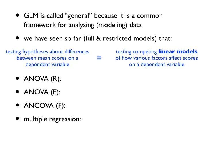
- GLM is called “general” because it is a common
framework for analysing (modeling) data
- we have seen so far (full & restricted models) that:
- ANOVA (R):
- ANOVA (F):
- ANCOVA (F):
- multiple regression:
testing hypotheses about differences between mean scores on a dependent variable testing competing linear models
- f how various factors affect scores
- n a dependent variable